TL;DR: there’s a Shiny app too.
I write this post as a follow-up to Erik Bernhardsson’s post “More MCMC – Analyzing a small dataset with 1-5 ratings.” Therein, Erik builds a simple multinomial regression to model explicit, 1-5 feedback scores for different variants of Better’s website. I like his approach for the rigor and mathematical fidelity it brings to what is a straightforward, ubiquitous use case for any product team.
I recently learned about ordered categorical generalized linear models (GLMs) and thought back to the post above. Of course, while feedback scores do fall into discrete categories, there is an implicit ordinality therein: choosing integers in ([1, 5]) is different from choosing colors in ({\text{red}, \text{green}, \text{blue}}). This is because 5 is greater than 4, while green is not “greater” than “blue.” (For a royalistic debate on the supremacy of the color green, please make use of the comments section below.)
In a multinomial regression, we can formulate our problem thus:
In a model with (k) categorical outcomes, we typically have (k-1) linear equations for (\phi_j). The link function — which you’ll recognize as the softmax — “squashes” these values such that they sum to 1 (with one of the values of (\phi_k) fixed at an arbitrary constant). The Normal priors placed on (\alpha) and (\beta) were chosen arbitrarily: we can use any continuous-valued distribution we like.
In situations where we don’t have predictor variables, we can alternatively draw the entire vector (p) from a Dirichlet distribution outright. As it happens, this offers us a trivially simple analytical solution to the posterior. This fact owes itself to Dirichlet-Multinomial conjugacy: given total observed counts (x_k) of each category (k) and respective parameters (\alpha_k) on our prior, our posterior distribution for our belief in (p) is given as:
This makes both inference and posterior predictive sampling trivial: a few lines of code for each. Unfortunately, while delightfully simple, the multinomial regression makes a strong concession with respect to the data at hand: the ordinality of our feedback scores is not explicitly preserved. To this effect, let us explore the ordered categorical GLM.
The ordered categorical GLM can be specified thus:
There’s a few components to clarify:
Ordered distribution
An Ordered distribution is a vanilla categorical distribution that accepts a vector of cumulative probabilities (p_k = \text{Pr}(y_i \leq k)), as opposed to traditional probabilities (p_k = \text{Pr}(y_i = k)). This preserves the ordering among variables.
Link function
In a typical logistic regression, we model the log-odds of observing a positive outcome as a linear function of the intercept plus weighted input variables. (The inverse of this function which we thereafter employ to obtain the raw probability (p) is the logistic function, or sigmoid function.) In the ordered categorical GLM, we instead model the log-cumulative-odds of observing a particular outcome as a linear function of the intercept minus weighted input variables. We’ll dive into the “minus” momentarily.
Cumulative probability
(p_k) in the above equation is defined as (p_k = \text{Pr}(y_i \leq k)). For this reason, the left-hand-side of the second line of our model gives the log-cumulative-odds, not the log-odds.
Priors
Placing Normal priors on (\alpha_k) and (\beta) was an arbitrary choice. In fact, any prior that produces a continuous value should suffice: the constraint that (p_k) must be a valid (cumulative) probability, i.e. (p_k) must lie on the interval ([0, 1]), is enforced by the inverse link function.
Subtracting (\phi_i)
Ultimately, (\phi_i) is the linear model. Should we want to add additional predictors, we would append them here. So, why do we subtract (\phi_i) from (\alpha_k) instead of add? Intuitively, it would make sense for an increase in the value of a predictor variable, given a positive coefficient, to shift probability mass towards larger ordinal values. This makes for a more fluid interpretation of our model parameters. Subtracting (\phi_i) does just this: increasing the value of a given predictor decreases the log-cumulative-odds of every outcome value (k) below the maximum (every outcome value below the maximum, because we have one linear model (\phi_i) which we must subtract, separately, from each intercept (\alpha_k) in order to compute (\log{\big(\frac{p_k}{1 - p_k}\big)})) which shifts probability mass upwards. This way, the desired dynamic — “a bigger predictor should lead to a bigger outcome given a positive coefficient” — holds.
Let’s move to R to fit and compare these models. I’m enjoying R more and more for the ease of plotting with ggplot2, as well as the functional “chains” offered by magrittr (“to be pronounced with a sophisticated french accent,” apparently) and Hadley Wickham’s dplyr.
First, let’s simulate some scores then plot the results.
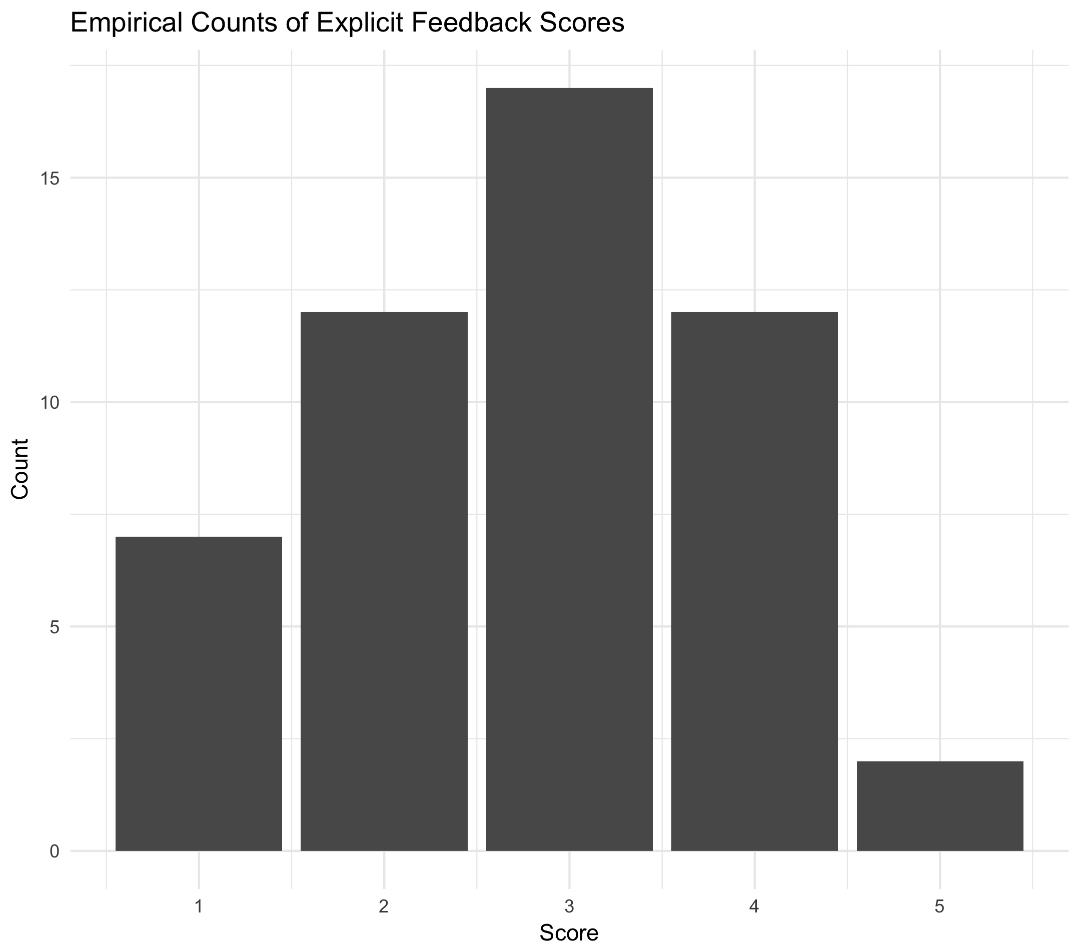
Next, let’s fit an ordered categorical GLM in the Stan modeling language. Note that we don’t have any predictor variables (x_i); therefore, the only variables we will be estimating are our intercepts (\alpha_k).
Our model estimates four values: (\alpha_1, \alpha_2, \alpha_3) and (\alpha_4). Why four and not five? The cumulative probability of the final outcome, (\text{Pr}(y_i \leq 5)) is always 1.
The posterior samples from our model will be vectors of cumulative probabilities, i.e. cumulative distribution functions. Let’s examine the variation in these estimates, and plot them against the proportion of each class observed in our original data to see how well our model did. The following plot is constructed with 2,000 samples from our posterior distribution, where each sample is given as ({\alpha_1, \alpha_2, \alpha_3, \alpha_4}). The dotted red line gives the column-wise mean, and the error band gives the column-wise 92% interval.
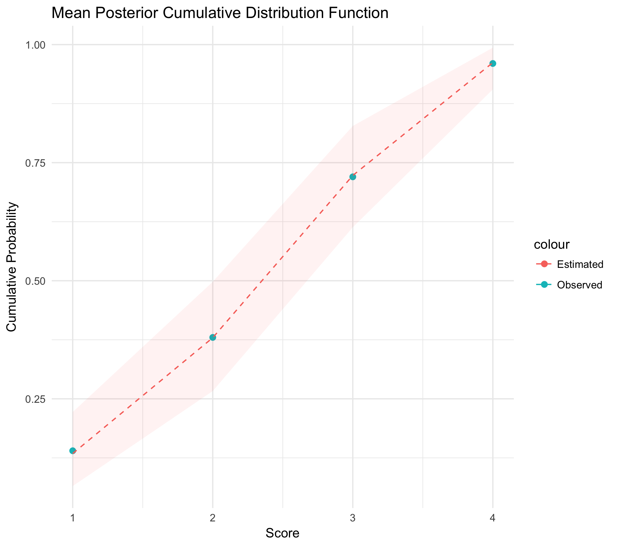
Key points are as follows:
The scale of our estimates
The marginal distributions of each estimated parameter are on the log-cumulative-odds scale. This is because (\alpha_k) — the only set of parameters we are estimating — is set equal to (\log{\bigg(\frac{\text{Pr}(y_i \leq k)}{1 - \text{Pr}(y_i \leq k)}\bigg)}) in our model above. So, what does a value of, say, (\alpha_3 = -1.5) say about the probability of receiving a feedback score of 3 from a given user? I have no idea. As such, we necessarily convert these estimates from the log-cumulative-odds scale to the cumulative probability scale to make interpretation easier. The sigmoid function gives this conversion.
The width of the band
The width of the band quantifies the uncertainty in our estimate of the true cumulative distribution function. We used 50 samples: it should be reasonably wide. With 500,000 samples, the red band would be indistinguishable from the dotted line.
Finally, let’s simulate new observations from each model. Our posterior contains a distribution of cumulative distribution functions: how do we translate this into multinomial samples?
First, samples from this distribution can be transformed into probability mass functions with the follow code:
Next, we can use each sample from simulated_probabilities to roll a multinomial die. Here, I’ll adopt the strategy Erik uses in the original post: with each sample, we’ll simulate a large number — I’ve chosen 500 — of multinomial throws. This will give a histogram of empirical counts — similar to the first plot shown at the top of this post. With this distribution, we’ll compute a weighted average. After repeating this for a large number of samples from our posterior, we’ll have a distribution of weighted averages. (Incidentally, as Erik highlights in his post, the shape of this distribution can be assumed Normal as given by the Central Limit Theorem.)
The following plot compares the results for both the ordered categorical and multinomial models. Remember, we obtain the posterior of the latter through the Dirichlet-Multinomial conjugacy described above. Sampling from this posterior follows trivially. While vanilla histograms should do the trick, let’s plot the inferred densities just to be safe.
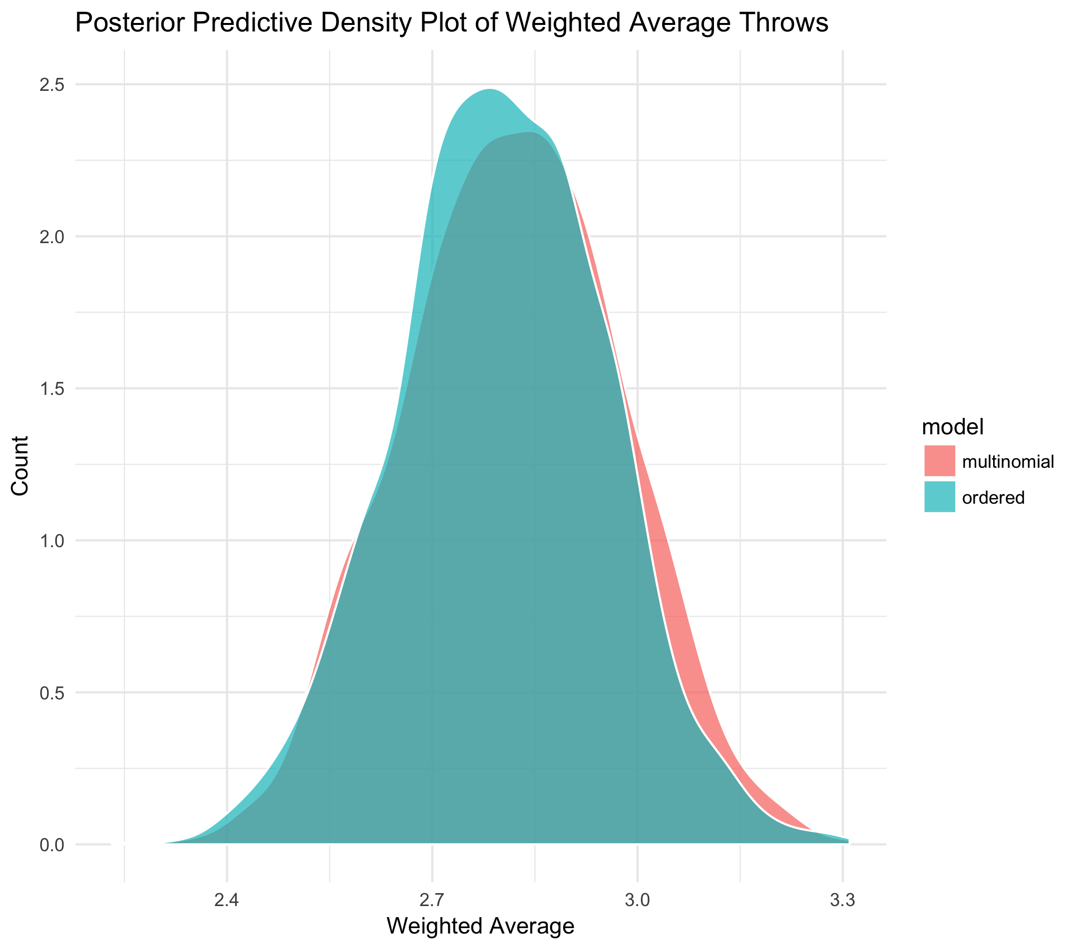
To be frank, this has me a little disappointed! According to the posterior predictive densities of the weighted-average throws, there is no discernible difference between the multinomial and ordered categorical models. To be thorough, let’s plot 100 draws from the raw, respective posteriors: a distribution over cumulative distribution functions for each model.
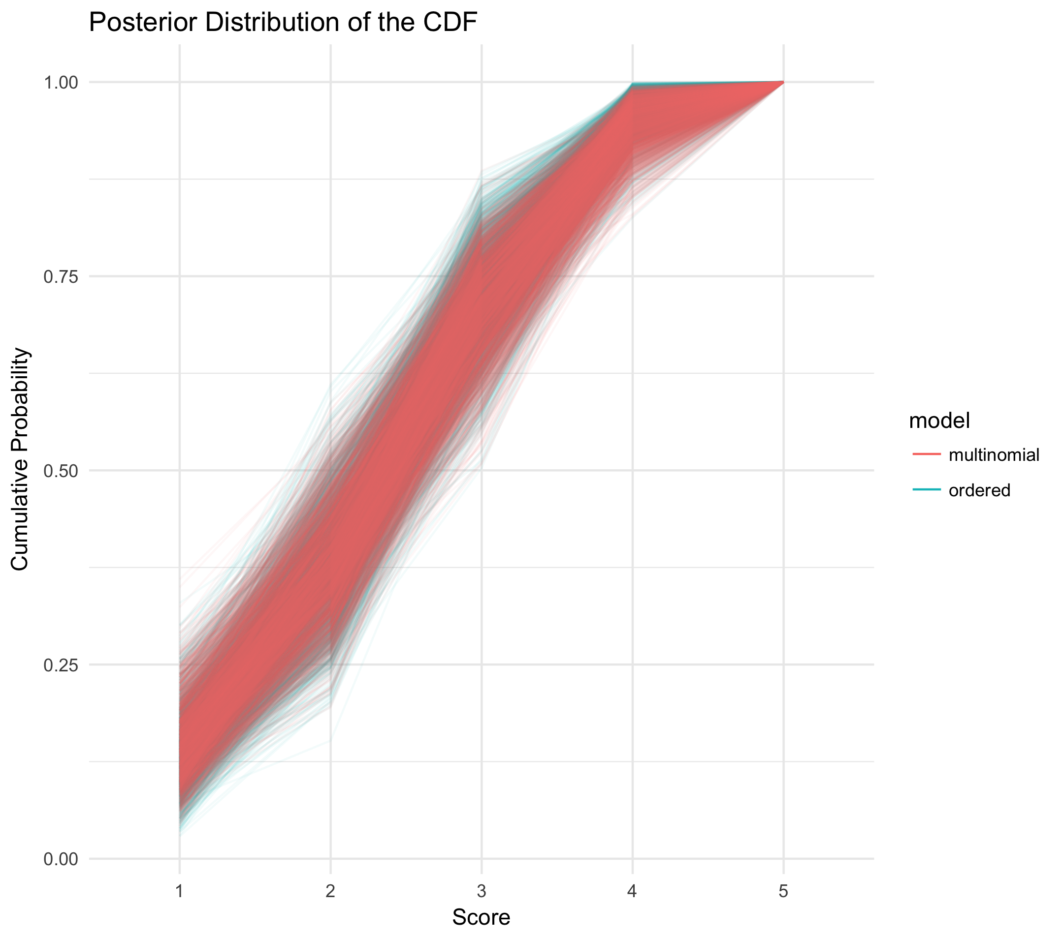
Yep, no difference. So, why do we think this is? What are our takeaways?
We didn’t use any predictor variables
In the ordered categorical case, we estimate (k - 1) values of (\alpha_k) and a single set of predictor coefficients. In the multinomial case, we estimate (k - 1) sets of ({\alpha_k, \beta_{X, k}}) values (for example, should we have (k = 3) classes and two predictor variables (a) and (b), we’d estimate parameters (\alpha_1, \beta_{a, 1}, \beta_{b, 1}, \alpha_{2}, \beta_{a, 2}, \beta_{b, 2}) in the simplest case). Given that we didn’t use any predictor variables, we’re simply estimating a set of intercepts (\alpha_k) in each case. In the former, these values give the log-cumulative-odds of each outcome, while in the latter they give the log-odds outright. Given that the transformation between the two is deterministic, the ordered categorical and multinomial models should be functionally identical.
We might want predictor variables
It is easy to conceive of a situation in which we’d want predictor variables. In this case, the ordered categorical model becomes a clear choice for ordered categorical data. Revisiting its formulation above, we see that predictors are trivial to add to the model: we just tack them onto the equation for (\phi_i).
The inconvenient realities of measurement
There’s a quote I like from Richard McElreath (I just finished his textbook, Statistical Rethinking, which I couldn’t recommend much more highly):
Both types of models help us transform our modeling to cope with the inconvenient realities of measurement, rather than transforming measurements to cope with the constraints of our models.
In this quote, he’s describing the ordered categorical GLM (in addition to “zero-inflated” models — models that “mix a binary event with an ordinary GLM likelihood like a Poisson or binomial” — hence the plurality). And therein lies the rub: a model is but an approximation of the world, and if one needs to bend to accommodate the other, the former should be preferred.
To conclude, I built a Shiny app to be used as an A/B test calculator for ordered categorical data using the methodologies detailed above. Example output looks as follows:
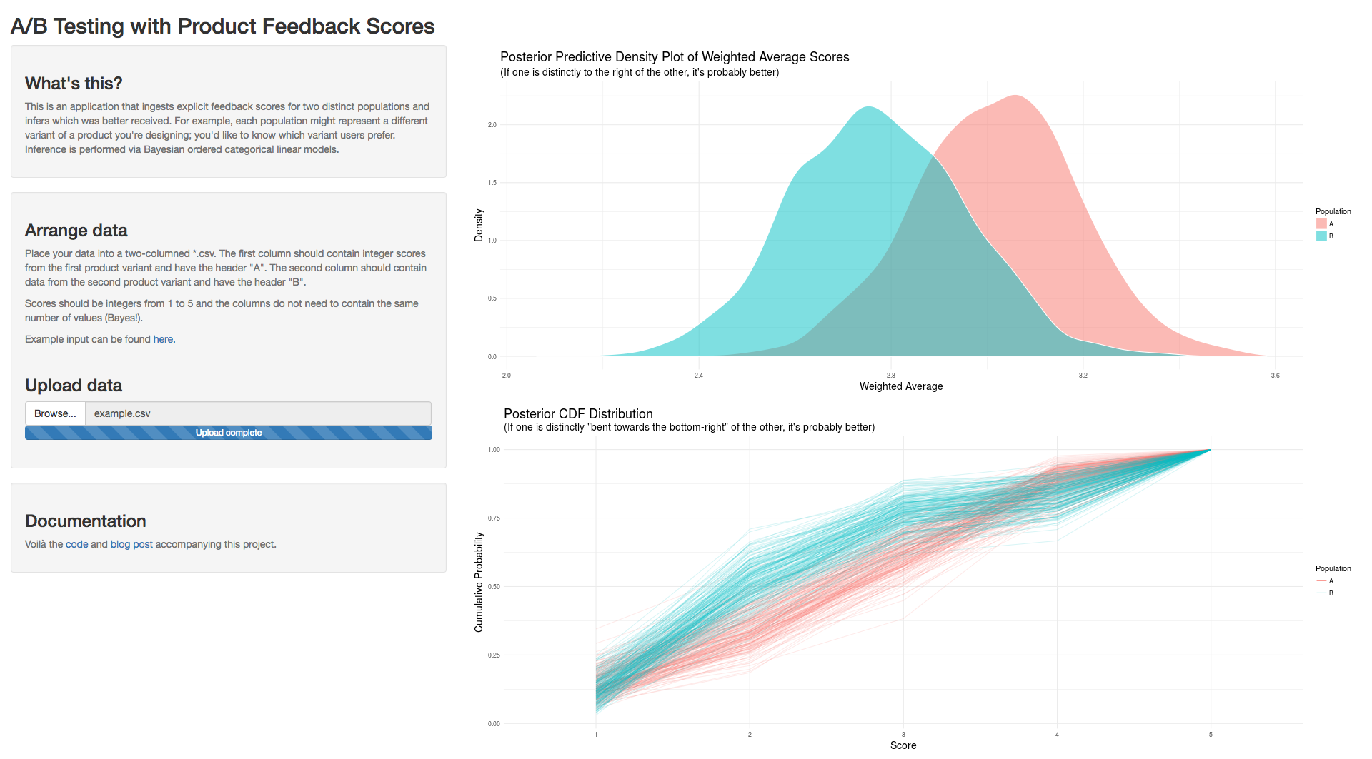
Code for this work can be found here. Thanks for reading.