The AUC score is a popular summary statistic that is often used to communicate the performance of a classifier. However, we illustrate here that this score depends not only on the quality of the model in question, but also on the difficulty of the test set considered: If samples are added to a test set that are easily classified, the AUC will go up — even if the model studied has not improved. In general, this behavior implies that isolated, single AUC scores cannot be used to meaningfully qualify a model’s performance. Instead, the AUC should be considered a score that is primarily useful for comparing and ranking multiple models — each at a common test set difficulty.
Follow us on twitter for new submission alerts!
Introduction
An important challenge associated with building good classification algorithms centers around their optimization: If an adjustment is made to an algorithm, we need a score that will enable us to decide whether or not the change made was an improvement. Many scores are available for this purpose. A sort-of all-purpose score that is quite popular for characterizing binary classifiers is the model AUC score (defined below).
The purpose of this post is to illustrate a subtlety associated with the AUC that is not always appreciated: The score depends strongly on the difficulty of the test set used to measure model performance. In particular, if any soft-balls are added to a test set that are easily classified (i.e., are far from any decision boundary), the AUC will increase. This increase does not imply a model improvement. Two key take-aways follow:
The AUC is an inappropriate score for comparing models validated on test sets having differing sampling distributions. Therefore, comparing the AUCs of models trained on samples having differing distributions requires care: The training sets can have different distributions, but the test sets must not. A single AUC measure cannot typically be used to meaningfully communicate the quality of a single model (though single model AUC scores are often reported!)
The primary utility of the AUC is that it allows one to compare multiple models at fixed test set difficulty: If a model change results in an increase in the AUC at fixed test set distribution, it can often be considered an improvement.
We review the definition of the AUC below and then demonstrate the issues alluded to above.
The AUC score, reviewed
Here, we quickly review the definition of the AUC. This is a score that can be used to quantify the accuracy of a binary classification algorithm on a given test set $\mathcal{S}$. The test set consists of a set of feature vector-label pairs of the form\begin{eqnarray}\tag{1}\mathcal{S} = {(\textbf{x}_i, y_i) }.\end{eqnarray}Here, $\textbf{x}_i$ is the set of features, or predictor variables, for example $i$ and $y_i \in {0,1 }$ is the label for example $i$. A classifier function $\hat{p}_1(\textbf{x})$ is one that attempts to guess the value of $y_i$ given only the feature vector $\textbf{x}_i$. In particular, the output of the function $\hat{p}_1(\textbf{x}_i)$ is an estimate for the probability that the label $y_i$ is equal to $1$. If the algorithm is confident that the class is $1$ ($0$), the probability returned will be large (small).
To characterize model performance, we can set a threshold value of $p^$ and mark all examples in the test set with $\hat{p}(\textbf{x}_i) > p^$ as being candidates for class one. The fraction of the truly positive examples in $\mathcal{S}$ marked in this way is referred to as the true-positive rate (TPR) at threshold $p^$. Similarly, the fraction of negative examples in $\mathcal{S}$ marked is referred to as the false-positive rate (FPR) at threshold $p^$. Plotting the TPR against the FPR across all thresholds gives the model’s so-called receiver operating characteristic (ROC) curve. A hypothetical example is shown at right in blue. The dashed line is just the $y=x$ line, which corresponds to the ROC curve of a random classifier (one returning a uniform random $p$ value each time).
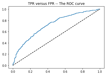
Notice that if the threshold is set to $p^* = 1$, no positive or negative examples will typically be marked as candidates, as this would require one-hundred percent confidence of class $1$. This means that we can expect an ROC curve to always go through the point $(0,0)$. Similarly, with $p^*$ set to $0$, all examples should be marked as candidates for class $1$ — and so an ROC curve should also always go through the point $(1,1)$. In between, we hope to see a curve that increases in the TPR direction more quickly than in the FPR direction — since this would imply that the examples the model is most confident about tend to actually be class $1$ examples. In general, the larger the Area Under the (ROC) Curve — again, blue at right — the better. We call this area the “AUC score for the model” — the topic of this post.
AUC sensitivity to test set difficulty
To illustrate the sensitivity of the AUC score to test set difficulty, we now consider a toy classification problem: In particular, we consider a set of unit-variance normal distributions, each having a different mean $\mu_i$. From each distribution, we will take a single sample $x_i$. From this, we will attempt to estimate whether or not the corresponding mean satisfies $\mu_i > 0$. That is, our training set will take the form $\mathcal{S} = {(x_i, \mu_i)}$, where $x_i \sim N(\mu_i, 1)$. For different $\mathcal{S}$, we will study the AUC of the classifier function,
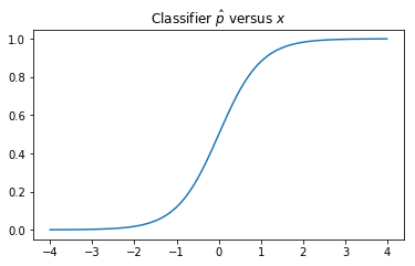
\begin{eqnarray} \label{classifier} \tag{2}\hat{p}(x) = \frac{1}{2} (1 + \text{tanh}(x))\end{eqnarray}A plot of this function is shown below. You can see that if any test sample $x_i$ is far to the right (left) of $x=0$, the model will classify the sample as positive (negative) with high certainty. At intermediate values near the boundary, the estimated probability of being in the positive class lifts in a reasonable way.
Notice that if a test example has a mean very close to zero, it will be difficult to classify that example as positive or negative. This is because both positive and negative $x$ samples are equally likely in this case. This means that the model cannot do much better than a random guess for such $\mu$. On the other hand, if an example $\mu$ is selected that is very far from the origin, a single sample $x$ from $N(\mu, 1)$ will be sufficient to make a very good guess as to whether $\mu > 0$. Such examples are hard to get wrong, soft-balls.
The impact of adding soft-balls to the test set on the AUC for model (\ref{classifier}) can be studied by changing the sampling distribution of $\mathcal{S}$. The following python snippet takes samples $\mu_i$ from three distributions — one tight about $0$ (resulting in a very difficult test set), one that is very wide containing many soft-balls that are easily classified, and one that is intermediate. The ROC curves that result from these three cases are shown following the code. The three curves are very different, with the AUC of the soft-ball set very large and that of the tight set close to that of the random classifier. Yet, in each case the model considered was the same — (\ref{classifier}). How could the AUC have improved?!
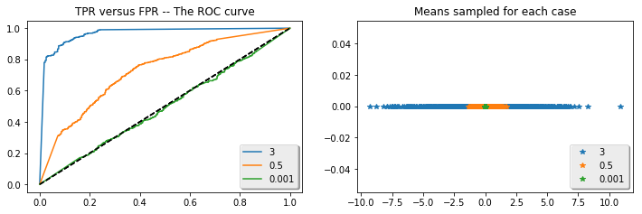
The explanation for the differing AUC values above is clear: Consider, for example, the effect of adding soft-ball negatives to $\mathcal{S}$. In this case, the model (\ref{classifier}) will be able to correctly identify almost all true positive examples at a much higher threshold than that where it begins to mis-classify the introduced negative softballs. This means that the ROC curve will now hit a TPR value of $1$ well-before the FPR does (which requires all negatives — including the soft-balls to be mis-classified). Similarly, if many soft-ball positives are added in, these will be easily identified as such well-before any negative examples are mis-classified. This again results in a raising of the ROC curve, and an increase in AUC — all without any improvement in the actual model quality, which we have held fixed.
Discussion
The toy example considered above illustrates the general point the AUC of a model is really a function of both the model and the test set it is being applied to. Keeping this in mind will help to prevent incorrect interpretations of the AUC. A special case to watch out for in practice is the situation where the AUC changes upon adjustment of the training and testing protocol applied (which can result, for example, from changes to how training examples are collected for the model). If you see such a change occur in your work, be careful to consider whether or not it is possible that the difficulty of the test set has changed in the process. If so, the change in the AUC may not indicate a change in model quality.
Because the AUC score of a model can depend highly on the difficulty of the test set, reporting this score alone will generally not provide much insight into the accuracy of the model — which really depends only on performance near the true decision boundary and not on soft-ball performance. Because of this, it may be a good practice to always report AUC scores for optimized models next to those of some fixed baseline model. Comparing the differences of the two AUC scores provides an approximate method for removing the effect of test set difficulty. If you come across an isolated, high AUC score in the wild, remember that this does not imply a good model!
A special situation exists where reporting an isolated AUC score for a single model can provide value: The case where the test set employed shares the same distribution as that of the application set (the space where the model will be employed). In this case, performance within the test set directly relates to expected performance during application. However, applying the AUC to situations such as this is not always useful. For example, if the positive class sits within only a small subset of feature space, samples taken from much of the rest of the space will be “soft-balls” — examples easily classified as not being in the positive class. Measuring the AUC on test sets over the full feature space in this context will always result in AUC values near one — leaving it difficult to register improvements in the model near the decision boundary through measurement of the AUC.