TLDR: In this blogpost, we’re going to train a neural network that is fully encrypted during training (trained on unencrypted data). The result will be a neural network with two beneficial properties. First, the neural network’s intelligence is protected from those who might want to steal it, allowing valuable AIs to be trained in insecure environments without risking theft of their intelligence. Secondly, the network can only make encrypted predictions (which presumably have no impact on the outside world because the outside world cannot understand the predictions without a secret key). This creates a valuable power imbalance between a user and a superintelligence. If the AI is homomorphically encrypted, then from it’s perspective, the entire outside world is also homomorphically encrypted. A human controls the secret key and has the option to either unlock the AI itself (releasing it on the world) or just individual predictions the AI makes (seems safer).

I typically tweet out new blogposts when they’re complete at @iamtrask. Feel free to follow if you’d be interested in reading more in the future and thanks for all the feedback!

Edit: If you’re interested in training Encrypted Neural Networks, check out the PySyft Library at OpenMined

Superintelligence

Many people are concerned that superpoweful AI will one day choose to harm humanity. Most recently, Stephen Hawking called for a new world government to govern the abilities that we give to Artificial Intelligence so that it doesn’t turn to destroy us. These are pretty bold statements, and I think they reflect the general concern shared between both the scientific community and the world at large. In this blogpost, I’d like to give a tutorial on a potential technical solution to this problem with some toy-ish example code to demonstrate the approach.

The goal is simple. We want to build A.I. technology that can become incredibly smart (smart enough to cure cancer, end world hunger, etc.), but whose intelligence is controlled by a human with a key, such that the application of intelligence is limited. Unlimited learning is great, but unlimited application of that knowledge is potentially dangerous.

To introduce this idea, I’ll quickly describe two very exciting fields of research: Deep Learning and Homomorphic Encryption.

Part 1: What is Deep Learning?

Deep Learning is a suite of tools for the automation of intelligence, primarily leveraging neural networks. As a field of computer science, it is largely responsible for the recent boom in A.I. technology as it has surpassed previous quality records for many intelligence tasks. For context, it played a big part in DeepMind’s AlphaGo system that recently defeated the world champion Go player, Lee Sedol.

Question: How does a neural network learn?

A neural network makes predictions based on input. It learns to do this effectively by trial and error. It begins by making a prediction (which is largely random at first), and then receives an “error signal” indiciating that it predicted too high or too low (usually probabilities). After this cycle repeats many millions of times, the network starts figuring things out. For more detail on how this works, see A Neural Network in 11 Lines of Python

The big takeaway here is this error signal. Without being told how well it’s predictions are, it cannot learn. This will be important to remember.

Part 2: What is Homomorphic Encryption?

As the name suggests, Homomorphic Encryption is a form of encryption. In the asymmetric case, it can take perfectly readable text and turn it into jibberish using a “public key”. More importantly, it can then take that jibberish and turn it back into the same text using a “secret key”. However, unless you have the “secret key”, you cannot decode the jibberish (in theory).

Homomorphic Encryption is a special type of encryption though. It allows someone to modify the encrypted information in specific ways * without being able to read the information*. For example, homomorphic encryption can be performed on numbers such that multiplication and addition can be performed on encrypted values without decrypting them. Here are a few toy examples.

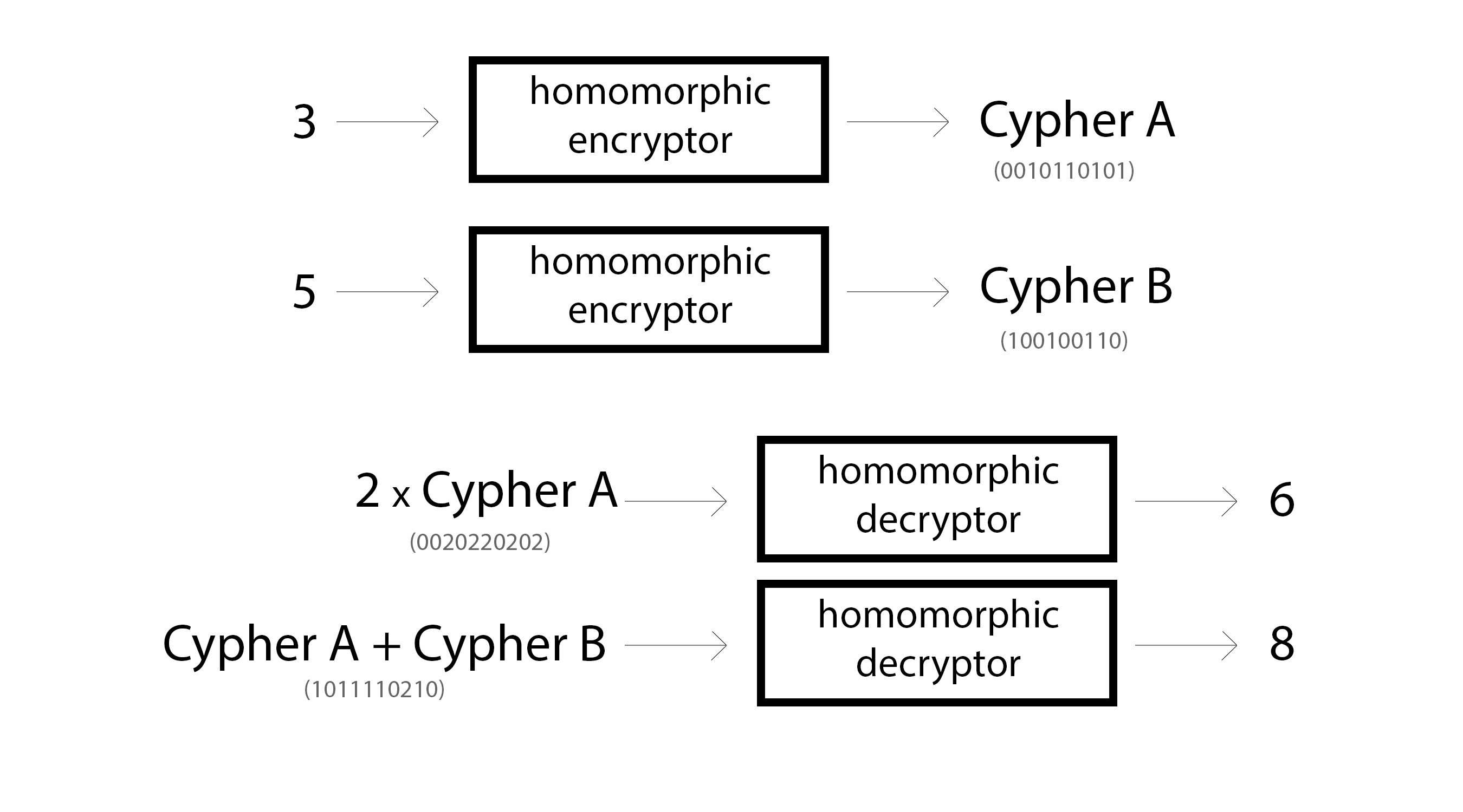
Now, there are a growing number of homomorphic encryption schemes, each with different properties. It’s a relatively young field and there are several significant problems still being worked through, but we’ll come back to that later.

For now, let’s just start with the following. Integer public key encryption schemes that are homomorphic over multiplication and addition can perform the operations in the picture above. Furthermore, because the public key allows for “one way” encryption, you can even perform operations between unencrypted numbers and encrypted numbers (by one-way encrypting them), as exemplified above by 2 * Cypher A. (Some encryption schemes don’t even require that… but again… we’ll come back to that later)

Part 3: Can we use them together?

Perhaps the most frequent intersection between Deep Learning and Homomorphic Encryption has manifested around Data Privacy. As it turns out, when you homomorphically encrypt data, you can’t read it but you still maintain most of the interesting statistical structure. This has allowed people to train models on encrypted data (CryptoNets). Furthermore a startup hedge fund called Numer.ai encrypts expensive, proprietary data and allows anyone to attempt to train machine learning models to predict the stock market. Normally they wouldn’t be able to do this becuase it would constitute giving away incredibly expensive information. (and normal encryption would make model training impossible)

However, this blog post is about doing the inverse, encrypting the neural network and training it on decrypted data.

A neural network, in all its amazing complexity, actually breaks down into a surprisingly small number of moving parts which are simply repeated over and over again. In fact, many state-of-the-art neural networks can be created using only the following operations:

So, let’s ask the obvious technical question, can we homomorphically encrypt the neural network itself? Would we want to? As it turns out, with a few conservative approximations, this can be done.

Addition - works out of the box
Multiplication - works out of the box
Division - works out of the box? - simply 1 / multiplication
Subtraction - works out of the box? - simply negated addition
Sigmoid - hmmm… perhaps a bit harder
Tanh - hmmm… perhaps a bit harder
Exponential - hmmm… perhaps a bit harder

It seems like we’ll be able to get Division and Subtraction pretty trivially, but these more complicated functions are… well… more complicated than simple addition and multiplication. In order to try to homomorphically encrypt a deep neural network, we need one more secret ingredient.

Part 4: Taylor Series Expansion

Perhaps you remember it from primary school. A Taylor Series allows one to compute a complicated (nonlinear) function using an infinite series of additions, subtractions, multiplications, and divisions. This is perfect! (except for the infinite part). Fortunately, if you stop short of computing the exact Taylor Series Expansion you can still get a close approximation of the function at hand. Here are a few popular functions approximated via Taylor Series (Source).

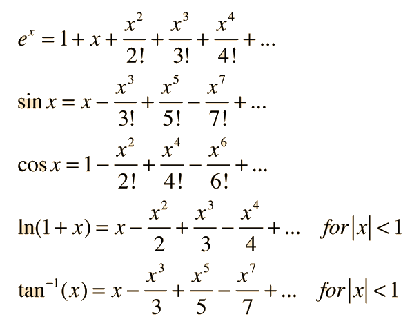
WAIT! THERE ARE EXPONENTS! No worries. Exponents are just repeated multiplication, which we can do. For something to play with, here’s a little python implementation approximating the Taylor Series for our desirable sigmoid function (the formula for which you can lookup on Wolfram Alpha). We’ll take the first few parts of the series and see how close we get to the true sigmoid function.

With only the first four factors of the Taylor Series, we get very close to sigmoid for a relatively large series of numbers. Now that we have our general strategy, it’s time to select a Homomorphic Encryption algorithm.

Part 5: Choosing an Encryption Algorithm

Homomorphic Encryption is a relatively new field, with the major landmark being the discovery of the first Fully Homomorphic algorithm by Craig Gentry in 2009. This landmark event created a foothold for many to follow. Most of the excitement around Homomorphic Encryption has been around developing Turing Complete, homomorphically encrypted computers. Thus, the quest for a fully homomorphic scheme seeks to find an algorithm that can efficiently and securely compute the various logic gates required to run arbitrary computation. The general hope is that people would be able to securely offload work to the cloud with no risk that the data being sent could be read by anyone other than the sender. It’s a very cool idea, and a lot of progress has been made.

However, there are some drawbacks. In general, most Fully Homomorphic Encryption schemes are incredibly slow relative to normal computers (not yet practical). This has sparked an interesting thread of research to limit the number of operations to be Somewhat homomorphic so that at least some computations could be performed. Less flexible but faster, a common tradeoff in computation.

This is where we want to start looking. In theory, we want a homomorphic encryption scheme that operates on floats (but we’ll settle for integers, as we’ll see) instead of binary values. Binary values would work, but not only would it require the flexibility of Fully Homomorphic Encryption (costing performance), but we’d have to manage the logic between binary representations and the math operations we want to compute. A less powerful, tailored HE algorithm for floating point operations would be a better fit.

Despite this constraint, there is still a plethora of choices. Here are a few popular ones with characteristics we like:

The best one to use here is likely either YASHE or FV. YASHE was the method used for the popular CryptoNets algorithm, with great support for floating point operations. However, it’s pretty complex. For the purpose of making this blogpost easy and fun to play around with, we’re going to go with the slightly less advanced (and possibly less secure) Efficient Integer Vector Homomorphic Encryption. However, I think it’s important to note that new HE algorithms are being developed as you read this, and the ideas presented in this blogpost are generic to any schemes that are homomorphic over addition and multiplication of integers and/or floating point numbers. If anything, it is my hope to raise awareness for this application of HE such that more HE algos will be developed to optimize for Deep Learning.

This encryption algorithm is also covered extensively by Yu, Lai, and Paylor in this work with an accompanying implementation here. The main bulk of the approach is in the C++ file vhe.cpp. Below we’ll walk through a python port of this code with accompanying explanation for what’s going on. This will also be useful if you choose to implement a more advanced scheme as there are themes that are relatively universal (general function names, variable names, etc.).

Part 6: Homomorphic Encryption in Python

Letâ€™s start by covering a bit of the Homomorphic Encryption jargon:

Plaintext: this is your un-encrypted data. It’s also called the “message”. In our case, this will be a bunch of numbers representing our neural network.
Cyphertext: this is your encrypted data. We’ll do math operations on the cyphertext which will change the underlying Plaintext.
Public Key: this is a pseudo-random sequence of numbers that allows anyone to encrypt data. It’s ok to share this with people because (in theory) they can only use it for encryption.
Private/Secret Key: this is a pseudo-random sequence of numbers that allows you to decrypt data that was encrypted by the Public Key. You do NOT want to share this with people. Otherwise, they could decrypt your messages.

So, those are the major moving parts. They also correspond to particular variables with names that are pretty standard across different homomorphic encryption techniques. In this paper, they are the following:

S: this is a matrix that represents your Secret/Private Key. You need it to decrypt stuff.
M: This is your public key. You’ll use it to encrypt stuff and perform math operations. Some algorithms don’t require the public key for all math operations but this one uses it quite extensively.
c: This vector is your encrypted data, your “cyphertext”.
x: This corresponds to your message, or your “plaintext”. Some papers use the variable “m” instead.
w: This is a single “weighting” scalar variable which we use to re-weight our input message x (make it consistently bigger or smaller). We use this variable to help tune the signal/noise ratio. Making the signal “bigger” makes it less susceptible to noise at any given operation. However, making it too big increases our likelihood of corrupting our data entirely. It’s a balance.
E or e: generally refers to random noise. In some cases, this refers to noise added to the data before encrypting it with the public key. This noise is generally what makes the decryption difficult. It’s what allows two encryptions of the same message to be different, which is important to make the message hard to crack. Note, this can be a vector or a matrix depending on the algorithm and implementation. In other cases, this can refer to the noise that accumulates over operations. More on that later.

As is convention with many math papers, capital letters correspond to matrices, lowercase letters correspond to vectors, and italic lowercase letters correspond to scalars.

Homomorphic Encryption has four kinds of operations that we care about: public/private keypair generation, one-way encryption, decryption, and the math operations. Let’s start with decryption.

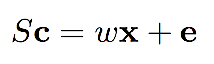
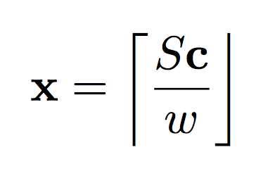
The formula on the left describes the general relationship between our secret key S and our message x. The formula on the right shows how we can use our secret key to decrypt our message. Notice that “e” is gone? Basically, the general philosophy of Homomorphic Encryption techniques is to introduce just enough noise that the original message is hard to get back without the secret key, but a small enough amount of noise that it amounts to a rounding error when you DO have the secret key. The brackets on the top and bottom represent “round to the nearest integer”. Other Homomorphic Encryption algorithms round to various amounts. Modulus operators are nearly ubiquitous.

Encryption, then, is about generating a c so that this relationship holds true. If S is a random matrix, then c will be hard to decrypt. The simpler, non-symmetric way of generating an encryption key is to just find the inverse of the secret key. Let’s start there with some Python code. –>

And when I run this code in an iPython notebook, I can perform the following operations (with corresponding output).

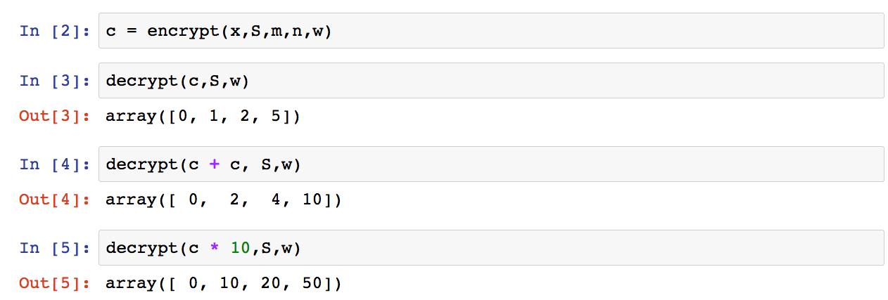
The key thing to look at are the bottom results. Notice that we can perform some basic operations to the cyphertext and it changes the underlying plaintext accordingly. Neat, eh?

Part 7: Optimizing Encryption

Import Lesson: Take a look at the decryption formulas again. If the secret key, S, is the identity matrix, then cyphertext c is just a re-weighted, slightly noisy version of the input x, which could easily be discovered given a handful of examples. If this doesn’t make sense, Google “Identity Matrix Tutorial” and come back. It’s a bit too much to go into here.

This leads us into how encryption takes place. Instead of explicitly allocating a self-standing “Public Key” and “Private Key”, the authors propose a “Key Switching” technique, wherein they can swap out one Private Key S for another S’. More specifically, this private key switching technique involves generating a matrix M that can perform the transformation.Since M has the ability to convert a message from being unencrypted (secret key of the identity matrix) to being encrypted (secret key that’s random and difficult to guess), this M becomes our public key!

That was a lot of information at a fast pace. Let’s nutshell that again. Here’s what happened…

Given the two formulas above, if the secret key is the identity matrix, the message isn’t encrypted.
Given the two formulas above, if the secret key is a random matrix, the generated message is encrypted.
We can make a matrix M that changes the secret key from one secret key to another.
When the matrix M converts from the identity to a random secret key, it is, by extension, encrypting the message in a one-way encryption.
Because M performs the role of a “one way encryption”, we call it the “public key” and can distribute it like we would a public key since it cannot decrypt the code.

So, without further adue, let’s see how this is done in Python.

import numpy as np

def generate_key(w,m,n): S = (np.random.rand(m,n) * w / (2 ** 16)) # proving max(S) < w return S

def encrypt(x,S,m,n,w): assert len(x) == len(S)

e = (np.random.rand(m)) # proving max(e) < w / 2 c = np.linalg.inv(S).dot((w * x) + e) return c

def decrypt(c,S,w): return (S.dot(c) / w).astype(‘int’)

def get_c_star(c,m,l): c_star = np.zeros(l * m,dtype=’int’) for i in range(m): b = np.array(list(np.binary_repr(np.abs(c[i]))),dtype=’int’) if(c[i] < 0): b *= -1 c_star[(i * l) + (l-len(b)): (i+1) * l] += b return c_star

def switch_key(c,S,m,n,T): l = int(np.ceil(np.log2(np.max(np.abs(c))))) c_star = get_c_star(c,m,l) S_star = get_S_star(S,m,n,l) n_prime = n + 1

S_prime = np.concatenate((np.eye(m),T.T),0).T A = (np.random.rand(n_prime - m, n*l) * 10).astype(‘int’) E = (1 * np.random.rand(S_star.shape[0],S_star.shape[1])).astype(‘int’) M = np.concatenate(((S_star - T.dot(A) + E),A),0) c_prime = M.dot(c_star) return c_prime,S_prime

def get_S_star(S,m,n,l): S_star = list() for i in range(l): S_star.append(S2**(l-i-1)) S_star = np.array(S_star).transpose(1,2,0).reshape(m,nl) return S_star

def get_T(n): n_prime = n + 1 T = (10 * np.random.rand(n,n_prime - n)).astype(‘int’) return T

def encrypt_via_switch(x,w,m,n,T): c,S = switch_key(x*w,np.eye(m),m,n,T) return c,S

x = np.array([0,1,2,5])

m = len(x) n = m w = 16 S = generate_key(w,m,n)

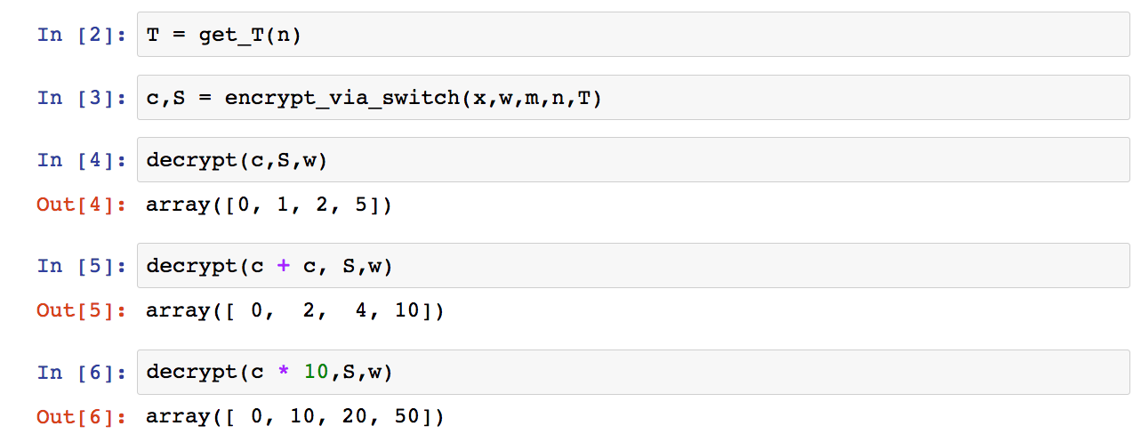
The way this works is by making the S key mostly the identiy matrix, simply concatenating a random vector T onto it. Thus, T really has all the information necessary for the secret key, even though we have to still create a matrix of size S to get things to work right.

Part 8: Building an XOR Neural Network

Floating Point Numbers: We’re going to do this by simply scaling our floats into integers. We’ll train our network on integers as if they were floats. Let’s say we’re scaling by 1000. 0.2 * 0.5 = 0.1. If we scale up, 200 * 500 = 100000. We have to scale down by 1000 twice since we performed multiplication, but 100000 / (1000 * 1000) = 0.1 which is what we want. This can be tricky at first but you’ll get used to it. Since this HE scheme rounds to the nearest integer, this also lets you control the precision of your neural net.
Vector-Matrix Multiplication: This is our bread and butter. As it turns out, the M matrix that converts from one secret key to another is actually a way to linear transform.
Inner Dot Product: In the right context, the linear transformation above can also be an inner dot product.
Sigmoid: Since we can do vector-matrix multiplication, we can evaluate arbitrary polynomials given enough multiplications. Since we know the Taylor Series polynomial for sigmoid, we can evaluate an approximate sigmoid!
Elementwise Matrix Multiplication: This one is surprisingly inefficient. We have to do a Vector-Matrix multiplication or a series of inner dot products.
Outer Product: We can accomplish this via masking and inner products.

Things to takeaway:

The weights of the network are all encrypted.
The data is decrypted… 1s and 0s.
After training, the network could be decrypted for increased performance or training (or switch to a different encryption key).
The training loss and output predictions are all also encrypted values. We have to decode them in order to be able to interpret the network.

Part 9: Sentiment Classification To make this a bit more real, here’s the same network training on IMDB sentiment reviews based on a network from Udacity’s Deep Learning Nanodegree. You can find the full code here

import time import sys import numpy as np

Let’s tweak our network from before to model these phenomena

class SentimentNetwork: def init(self, reviews,labels,min_count = 10,polarity_cutoff = 0.1,hidden_nodes = 8, learning_rate = 0.1): np.random.seed(1234) self.pre_process_data(reviews, polarity_cutoff, min_count) self.init_network(len(self.review_vocab),hidden_nodes, 1, learning_rate)

def pre_process_data(self,reviews, polarity_cutoff,min_count): print(“Pre-processing data…”)

positive_counts = Counter() negative_counts = Counter() total_counts = Counter()

for i in range(len(reviews)): if(labels[i] == ‘POSITIVE’): for word in reviews[i].split(“ “): positive_counts[word] += 1 total_counts[word] += 1 else: for word in reviews[i].split(“ “): negative_counts[word] += 1 total_counts[word] += 1

pos_neg_ratios = Counter()

for term,cnt in list(total_counts.most_common()): if(cnt >= 50): pos_neg_ratio = positive_counts[term] / float(negative_counts[term]+1) pos_neg_ratios[term] = pos_neg_ratio

for word,ratio in pos_neg_ratios.most_common(): if(ratio > 1): pos_neg_ratios[word] = np.log(ratio) else: pos_neg_ratios[word] = -np.log((1 / (ratio + 0.01)))

review_vocab = set() for review in reviews: for word in review.split(“ “): if(total_counts[word] > min_count): if(word in pos_neg_ratios.keys()): if((pos_neg_ratios[word] >= polarity_cutoff) or (pos_neg_ratios[word] <= -polarity_cutoff)): else: review_vocab.add(word) self.review_vocab = list(review_vocab)

label_vocab = set() for label in labels: label_vocab.add(label) self.label_vocab = list(label_vocab)

self.review_vocab_size = len(self.review_vocab) self.label_vocab_size = len(self.label_vocab)

self.word2index = {} for i, word in enumerate(self.review_vocab): self.word2index[word] = i

self.label2index = {} for i, label in enumerate(self.label_vocab): self.label2index[label] = i

def init_network(self, input_nodes, hidden_nodes, output_nodes, learning_rate): # Set number of nodes in input, hidden and output layers. self.input_nodes = input_nodes self.hidden_nodes = hidden_nodes self.output_nodes = output_nodes

print(“Initializing Weights…”) self.weights_0_1_t = np.zeros((self.input_nodes,self.hidden_nodes))

self.weights_1_2_t = np.random.normal(0.0, self.output_nodes**-0.5, (self.hidden_nodes, self.output_nodes))

print(“Encrypting Weights…”) self.weights_0_1 = list() for i,row in enumerate(self.weights_0_1_t): sys.stdout.write(“\rEncrypting Weights from Layer 0 to Layer 1:” + str(float((i+1) * 100) / len(self.weights_0_1_t))[0:4] + “% done”) self.weights_0_1.append(one_way_encrypt_vector(row,scaling_factor).astype(‘int64’)) print(“”)

self.weights_1_2 = list() for i,row in enumerate(self.weights_1_2_t): sys.stdout.write(“\rEncrypting Weights from Layer 1 to Layer 2:” + str(float((i+1) * 100) / len(self.weights_1_2_t))[0:4] + “% done”) self.weights_1_2.append(one_way_encrypt_vector(row,scaling_factor).astype(‘int64’)) self.weights_1_2 = transpose(self.weights_1_2) self.learning_rate = learning_rate

self.layer_0 = np.zeros((1,input_nodes)) self.layer_1 = np.zeros((1,hidden_nodes))

def sigmoid(self,x): return 1 / (1 + np.exp(-x))

def sigmoid_output_2_derivative(self,output): return output * (1 - output)

def update_input_layer(self,review):

# clear out previous state, reset the layer to be all 0s self.layer_0 *= 0 for word in review.split(“ “): self.layer_0[0][self.word2index[word]] = 1

def get_target_for_label(self,label): if(label == ‘POSITIVE’): return 1 else: return 0

def train(self, training_reviews_raw, training_labels):

training_reviews = list() for review in training_reviews_raw: indices = set() for word in review.split(“ “): if(word in self.word2index.keys()): indices.add(self.word2index[word]) training_reviews.append(list(indices))

layer_1 = np.zeros_like(self.weights_0_1[0])

start = time.time() correct_so_far = 0 total_pred = 0.5 for i in range(len(training_reviews_raw)): review_indices = training_reviews[i] label = training_labels[i]

layer_1 *= 0 for index in review_indices: layer_1 += self.weights_0_1[index] layer_1 = layer_1 / float(len(review_indices)) layer_1 = layer_1.astype(‘int64’) # round to nearest integer

layer_2 = sigmoid(innerProd(layer_1,self.weights_1_2[0],M_onehot[len(layer_1) - 2][1],l) / float(scaling_factor))[0:2]

if(label == ‘POSITIVE’): layer_2_delta = layer_2 - (c_ones[len(layer_2) - 2] * scaling_factor) else: layer_2_delta = layer_2

weights_1_2_trans = transpose(self.weights_1_2) layer_1_delta = mat_mul_forward(layer_2_delta,weights_1_2_trans,scaling_factor).astype(‘int64’)

self.weights_1_2 -= np.array(outer_product(layer_2_delta,layer_1)) * self.learning_rate

for index in review_indices: self.weights_0_1[index] -= (layer_1_delta * self.learning_rate).astype(‘int64’)

# we’re going to decrypt on the fly so we can watch what’s happening total_pred += (s_decrypt(layer_2)[0] / scaling_factor) if((s_decrypt(layer_2)[0] / scaling_factor) >= (total_pred / float(i+2)) and label == ‘POSITIVE’): if((s_decrypt(layer_2)[0] / scaling_factor) < (total_pred / float(i+2)) and label == ‘NEGATIVE’): correct_so_far += 1

reviews_per_second = i / float(time.time() - start)

sys.stdout.write(“\rProgress:” + str(100 * i/float(len(training_reviews_raw)))[:4] + “% Speed(reviews/sec):” + str(reviews_per_second)[0:5] + “ #Correct:” + str(correct_so_far) + “ #Trained:” + str(i+1) + “ Training Accuracy:” + str(correct_so_far * 100 / float(i+1))[:4] + “%”) if(i % 100 == 0): print(i)

def test(self, testing_reviews, testing_labels): correct = 0 start = time.time()

for i in range(len(testing_reviews)): pred = self.run(testing_reviews[i]) if(pred == testing_labels[i]): correct += 1 reviews_per_second = i / float(time.time() - start)

sys.stdout.write(“\rProgress:” + str(100 * i/float(len(testing_reviews)))[:4] \

”% Speed(reviews/sec):” + str(reviews_per_second)[0:5] \
”% #Correct:” + str(correct) + “ #Tested:” + str(i+1) + “ Testing Accuracy:” + str(correct * 100 / float(i+1))[:4] + “%”) def run(self, review):

# Input Layer

# Hidden layer self.layer_1 *= 0 unique_indices = set() for word in review.lower().split(“ “): if word in self.word2index.keys(): unique_indices.add(self.word2index[word]) for index in unique_indices: self.layer_1 += self.weights_0_1[index]

# Output layer layer_2 = self.sigmoid(self.layer_1.dot(self.weights_1_2))

if(layer_2[0] >= 0.5): return “POSITIVE” else: return “NEGATIVE”

Progress:0.0% Speed(reviews/sec):0.0 #Correct:1 #Trained:1 Training Accuracy:100.%0 Progress:0.41% Speed(reviews/sec):1.978 #Correct:66 #Trained:101 Training Accuracy:65.3%100 Progress:0.83% Speed(reviews/sec):2.014 #Correct:131 #Trained:201 Training Accuracy:65.1%200 Progress:1.25% Speed(reviews/sec):2.011 #Correct:203 #Trained:301 Training Accuracy:67.4%300 Progress:1.66% Speed(reviews/sec):2.003 #Correct:276 #Trained:401 Training Accuracy:68.8%400 Progress:2.08% Speed(reviews/sec):2.007 #Correct:348 #Trained:501 Training Accuracy:69.4%500 Progress:2.5% Speed(reviews/sec):2.015 #Correct:420 #Trained:601 Training Accuracy:69.8%600 Progress:2.91% Speed(reviews/sec):1.974 #Correct:497 #Trained:701 Training Accuracy:70.8%700 Progress:3.33% Speed(reviews/sec):1.973 #Correct:581 #Trained:801 Training Accuracy:72.5%800 Progress:3.75% Speed(reviews/sec):1.976 #Correct:666 #Trained:901 Training Accuracy:73.9%900 Progress:4.16% Speed(reviews/sec):1.983 #Correct:751 #Trained:1001 Training Accuracy:75.0%1000 Progress:4.33% Speed(reviews/sec):1.940 #Correct:788 #Trained:1042 Training Accuracy:75.6% ….

Part 10: Advantages over Data Encryption The most similar approach to this one is to encrypt training data and train neural networks on the encrypted data (accepting encrypted input and predicting encrypted output). This is a fantastic idea. However, it does have a few drawbacks. First and foremost, encrypting the data means that the neural network is completely useless to anyone without the private key for the encrypted data. This makes it impossible for data from different private sources to be trained on the same Deep Learning model. Most commercial applications have this requirement, requiring the aggregation of consumer data. In theory, we’d want every consumer to be protected by their own secret key, but homomorphically encrypting the data requires that everyone use the SAME key.

Part 10: Advantages over Data Encryption

However, encrypting the network doesn’t have this restriction.

With the approach above, you could train a regular, decrypted neural network for a while, encrypt it, send it to Party A with a public key (who trains it for a while on their own data… which remains in their possession). Then, you could get the network back, decrypt it, re-encrypt it with a different key and send it to Party B who does some training on their data. Since the network itself is what’s enrypted, you get total control over the intelligence that you’re capturing along the way. Party A and Party B would have no way of knowing that they each received the same network, and this all happens without them ever being able to see or use the network on their own data. You, the company, retain control over the IP in the neural network, and each user retains control over their own data.

Part 11: Future Work

Part 12: Potential Applications

Decentralized AI: Companies can deploy models to be trained or used in the field without risking their intelligence being stolen.

Protected Consumer Privacy: the previous application opens up the possibility that consumers could simply hold onto their data, and “opt in” to different models being trained on their lives, instead of sending their data somewhere else. Companies have less of an excuse if their IP isn’t at risk via decentralization. Data is power and it needs to go back to the people.

Controlled Superintelligence: The network can become as smart as it wants, but unless it has the secret key, all it can do is predict jibberish.

Building Safe A.I.

未知