In the previous parts of the series we demonstrated a positive results bias in optimism corrected bootstrapping by simply adding random features to our labels. This problem is due to an ‘information leak’ in the algorithm, meaning the training and test datasets are not kept seperate when estimating the optimism. Due to this, the optimism, under some conditions, can be very under estimated. Let’s analyse the code, it is pretty straightforward to understand then we can see where the problem originates.
- Fit a model M to entire data S and estimate predictive ability C. ## this part is our overfitted estimation of performance (can be AUC, accuracy, etc)
Iterate from b=1…B: ## now we are doing resampling of the data to estimate the error
-
Take a resample from the original data, S*
-
Fit the bootstrap model M* to S* and get predictive ability, C_boot ## this will clearly give us another overfitted model performance, which is fine
-
Use the bootstrap model M* to get predictive ability on S, C_orig ## we are using the same data (samples) used to train the model to test it, therefore it is not surprising that we have values with better performance than expected. C_orig values will be too high.
One way of correcting for this would be changing step 3 of the bootstrap, instead of testing on the original data, to test on the left out (unseen) data in the bootstrap. This way the training and test data is kept entirely seperate in terms of samples, thus eliminating our bias towards inflated model performance on null datasets with high features. There is probably no point of doing anyway this when we have methods such as LOOCV and K fold cross validation.
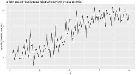
As p (features) » N (samples) we are going to get better and better ability to get good model performance using the bootstrapped data on the original data. Why? Because the original data contains the same samples as the bootstrap and as we get more features, greater the chance we are going to get some randomly correlating with our response variable. When we test the bootstrap on the original data (plus more samples) it retains some of this random ability to predict the real labels. This is a typical overfitting problem when we have higher numbers of features, and the procedure is faulty.
Let’s take another experimental look at the problem, this code can be directly copied and pasted into R for repeating the analyses and plots. We have two implementations of the method, the first by me for glmnet (lasso logisitic regression), the second for glm (logisitic regression) from this website (http://cainarchaeology.weebly.com/r-function-for-optimism-adjusted-auc.html). Feel free to try different machine learning algorithms and play with the parameters.
So here are the results, as number of noise only features on the x axis increase our ‘corrected’ estimate of AUC (on y axis) also increases when we start getting enough to allow that noise to randomly predict the labels. So this shows the problem starts about 40-50 features, then gets worse until about 75+. This is with the ‘glmnet’ function.


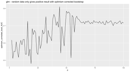
Let’s look at the method using glm, we find the same trend, different implementation.
So there we have it, the method has a problem with it and should not be used with greater than about 40 features. This method unfortunately is currently being used for datasets with higher than this number of dimensions (40+) because people think it is a published method it is safe, unfortunately this is not how the world works R readers. Remember, the system is corrupt, science and statistics is full of lies, and if in doubt, do your own tests on positive and negative controls.
This is with the ‘glm’ function. Random features added on x axis, the corrected AUC on y axis.


What if you don’t believe it? I mean this is a text book method. Well R readers if that is so I suggest code it your self and try the code here, run the experiments on null (random data only) datasets with increasing features.
This is the last part in the series on debunking the optimism corrected bootstrap method. I consider it, debunked.
Related