Thanks a lot to @aerinykim, @suzatweet and @hardmaru for the useful feedback!
The academic Deep Learning research community has largely stayed away from the financial markets. Maybe that’s because the finance industry has a bad reputation, the problem doesn’t seem interesting from a research perspective, or because data is difficult and expensive to obtain.
In this post, I’m going to argue that training Reinforcement Learning agents to trade in the financial (and cryptocurrency) markets can be an extremely interesting research problem. I believe that it has not received enough attention from the research community but has the potential to push the state-of-the art of many related fields. It is quite similar to training agents for multiplayer games such as DotA, and many of the same research problems carry over. Knowing virtually nothing about trading, I have spent the past few months working on a project in this field.
This is not a “price prediction using Deep Learning” post. So, if you’re looking for example code and models you may be disappointed. Instead, I want to talk on a more high level about why learning to trade using Machine Learning is difficult, what some of the challenges are, and where I think Reinforcement Learning fits in. If there’s enough interest in this area I may follow up with another post that includes concrete examples.
I expect most readers to have no background in trading, just like I didn’t, so I will start out with covering some of the basics. I’m by no means an expert, so please let me know in the comments so if you find mistakes. I will use cryptocurrencies as a running example in this post, but the same concepts apply to most of the financial markets. The reason to use cryptocurrencies is that data is free, public, and easily accessible. Anyone can sign up to trade. The barriers to trading in the financial markets are a little higher, and data can be expensive. And well, there’s more hype so it’s more fun :)
Basics of Market Microstructure
Trading in the cryptocurrency (and most financial) markets happens in what’s called a continuous double auction with an open order book on an exchange. That’s just a fancy way of saying that there are buyers and sellers that get matched so that they can trade with each other. The exchange is responsible for the matching. There are dozens of exchanges and each may carry slightly different products (such as Bitcoin or Ethereum versus U.S. Dollar). Interface-wise, and in terms of the data they provide, they all look pretty much the same.
Let’s take a look at GDAX, one of the more popular U.S.-based exchanges. Let’s assume you want to trade BTC-USD (Bitcoin for U.S. Dollar). You would go to this page and see something like this:
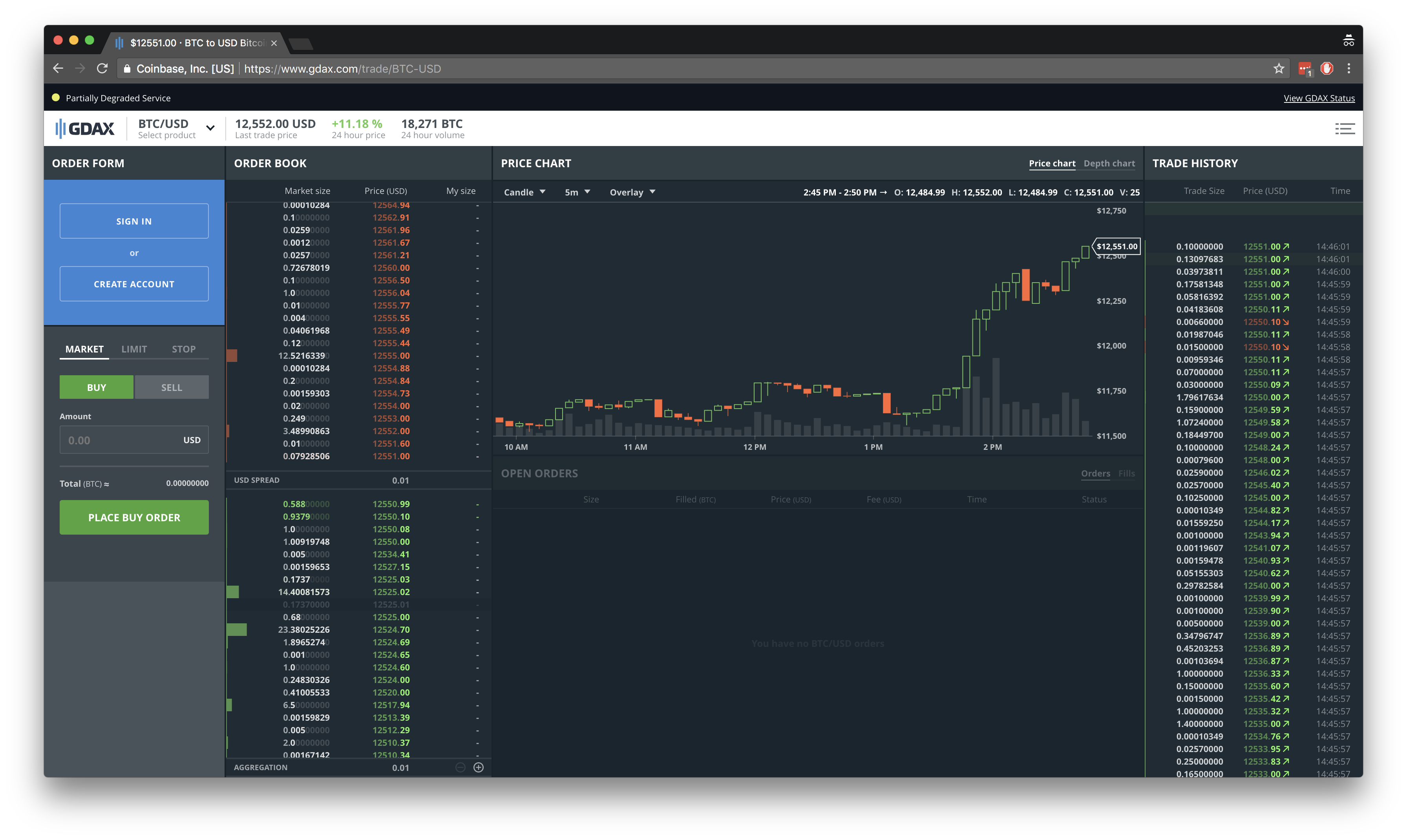
There’s a lot of information here, so let’s go over the basics:
Price chart (Middle)
The current price is the price of the most recent trade. It varies depending on whether that trade was a buy or a sell (more on that below). The price chart is typically displayed as a candlestick chart that shows the Open/Start (O), High (H), Low (L) and Close/End (C) prices for a given time window. In the picture above, that period is 5 minutes, but you can change it using the dropdown. The bars below the price chart show the Volume (V), which is the total volume of all trades that happened in that period. The volume is important because it gives you a sense of the liquidity of the market. If you want to buy $100,000 worth if Bitcoin, but there is nobody willing to sell, the market is illiquid. You simply can’t buy. A high trade volume indicates that many people are willing to transact, which means that you are likely to able to buy or sell when you want to do so. Generally speaking, the more money you want to invest, the more trade volume you want. Volume also indicates the “quality” of a price trend. High volume means you can rely on the price movement more than if there was low volume. High volume is often (but not always, as in the case of market manipulation) the consensus of a large number of market participants.
Trade History (Right)
The right side shows a history of all recent trades. Each trade has a size, price, timestamp, and direction (buy or sell). A trade is a match between two parties, a taker and a maker. More on that below.
Order Book (Left)
The left side shows the order book, which contains information about who is willing to buy and sell at what price. The order book is made up of two sides: Asks (also called offers), and Bids. Asks are people willing to sell, and bids are people willing to buy. By definition, the best ask, the lowest price that someone is willing to sell at, is larger than the best bid, the highest price that someone is willing to buy at. If this was not the case, a trade between these two parties would’ve already happened. The difference between the best ask and best bid is called the spread.
Each level of the order book has a price and a volume. For example, a volume of 2.0 at a price level of $10,000 means that you can buy 2 BTC for $10,000. If you want to buy more, you would need to pay a higher price for the amount that exceeds 2 BTC. The volume at each level is cumulative, which means that you don’t know how many people, or orders, that 2 BTC consists of. There could one person selling 2 BTC, or there could be 100 people selling 0.02 BTC each (some exchanges provide this level of information, but most don’t). Let’s look at an example:
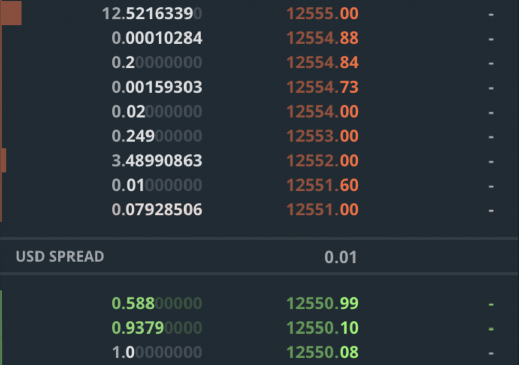
So what happens when you send an order to buy 3 BTC? You would be buying (rounding up) 0.08 BTC at $12,551.00, 0.01BTC at $12,551.6 and 2.91 BTC at $12,552.00. On GDAX, you would also be paying a 0.3% taker fee, for a total of about 1.003 * (0.08 * 12551 + 0.01 * 12551.6 + 2.91 * 12552) = $37,768.88 and an average price per BTC of 37768.88 / 3 = $12,589.62. It’s important to note that what you are actually paying is much higher than $12,551.00, which was the current price! The 0.3% fee on GDAX is extremely high compared to fees in the financial markets, and also much higher than the fees of many other cryptocurrency exchanges, which are often between 0% and 0.1%.
Also note that your buy order has consumed all the volume that was available at the $12,551.00 and $12,551.60 levels. Thus, the order book will “move up”, and the best ask will become $12,552.00. The current price will also become $12,552.00, because that is where the last trade happened. Selling works analogously, just that you are now operating on the bid side of the order book, and potentially moving the order book (and price) down. In other words, by placing buy and sell orders, you are removing volume from the order book. If your orders are large enough, you may shift the order book by several levels. In fact, if you placed a very large order for a few million dollars, you would shift the order book and price significantly.
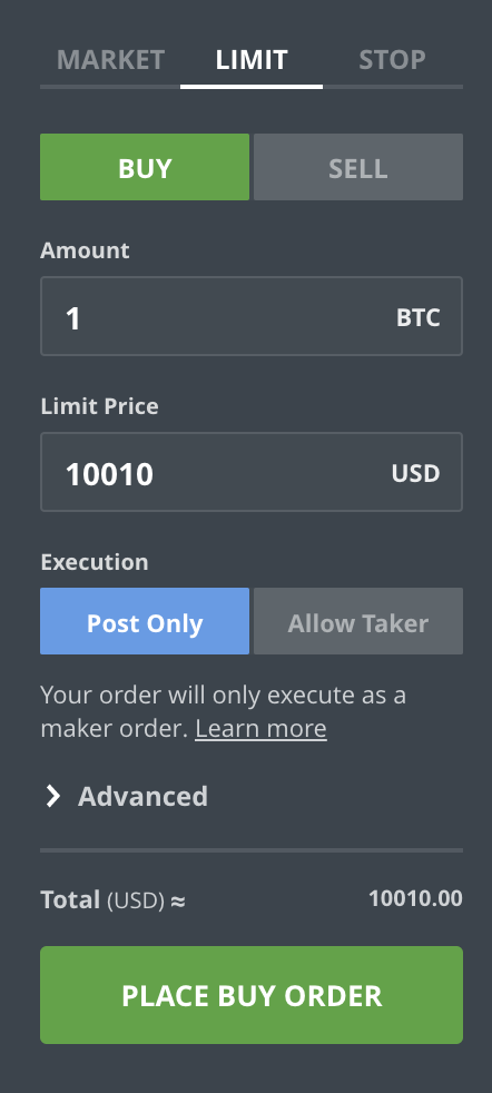
How do orders get into the order book? That’s the difference between market and limit orders. In the above example, you’ve issued a market order, which basically means “Buy/Sell X amount of BTC at the best price possible, right now“. If you are not careful about what’s in the order book you could end up paying significantly more than the current price shows. For example, imagine that most of the lower levels in the order book only had a volume at 0.001 BTC available. Most of your buy volume would then get matched at a much higher, more expensive, price level. If you submit a limit order, also called a passive order, you specify the price and quantity you’re willing to buy or sell at. The order will be placed into the book, and you can cancel it as long as it has not been matched. For example, let’s assume the Bitcoin price is at $10,000, but you want to sell at $10,010. You place a limit order. First, nothing happens. If the price keeps moving down your order will just sit there, do nothing, and will never be matched. You can cancel it anytime. However, if the price moves up, your order will at some point become the best price in the book, and the next person submitting a market order for a sufficient quantity will match it.
Market orders take liquidity from the market. By matching with orders from the order book, you are taking away the option to trade to from other people – there’s less volume left! That’s also why market orders, or market takers, often need to pay higher fees than* market makers, who put orders into the book. Limit orders providing liquidity* because they are giving others the option to trade. At the same time, limit orders guarantee that you will not pay more than the price specified in the limit order. However, you don’t know when, or if, someone will match your order. You are also giving the market information about what you believe the price should be. This can also be used to manipulate the other participants in the market, who may act a certain way based on the orders you are executing or putting into the book. Because they provide the option to trade and give away information, market makers typically pay lower fees than market takers. Some exchanges also provide stop orders, which allow you to set a maximum price for your market orders.
This was a very short introduction of how order books works and matching works. There are many more subtleties as well other, much more complex, order types. If the above was not clear, you can find a wealth of information about order book mechanics, and research in that area, through Google.
Data
The main reasons I am using cryptocurrencies in this post is because data is public, free, and easy to obtain. Most exchanges have streaming APIs that allow you to receive market updates in real-time. We’ll use GDAX (API Documentation) as an example again, but the data for other exchanges looks very similar. Let’s go over the basic types of events you would use to build a Machine Learning model.
Trade
A new Trade has happened. Each trade has a timestamp, a unique ID assigned by the exchange, a price, size, and side, as discussed above. If you wanted to plot the price graph of an asset, you would simply plot the price of all trades. If you wanted to plot the candlestick chart, you would window the trade events for a certain period, such as five minutes, and then plot the windows.
BookUpdate
One or more levels in the order book were updated. Each level is made up of the side (Buy=Bid, Sell=Ask), the price/level, and the new quantity at that level. Note that these are changes, or deltas, and you must construct the full order book yourself by merging them.
BookSnapshot
Similar to a BookUpdate, but a snapshot of the complete order book. Because the full order book can be very large, it is faster and more efficient to use the BookUpdate events instead. However, having an occasional snapshot can be useful.
That’s pretty much all you need in terms of market data. A stream of the above events contains all the information you saw in the GUI interface. You can imagine how you could make prediction based on a stream of the above events.
A few Trading Strategy Metrics
When developing trading algorithms, what do you optimize for? The obvious answer is profit, but that’s not the whole story. You also need to compare your trading strategy to baselines, and compare its risk and volatility to other investments. Here are a few of the most basic metrics that traders are using. I won’t go into detail here, so feel free to follow the links for more information.
Net PnL (Net Profit and Loss)
Simply how much money an algorithm makes (positive) or loses (negative) over some period of time, minus the trading fees.
Alpha and Beta
Alpha defines how much better, in terms of profit, your strategy is when compared to an alternative, relatively risk-free, investment, like a government bond. Even if your strategy is profitable, you could be better off investing in a risk-free alternative. Beta is closely related, and tells you how volatile your strategy is compared to the market. For example, a beta of 0.5 means that your investment moves $1 when the market moves $2.
Sharpe Ratio
The Sharpe Ratio measures the excess return per unit of risk you are taking. It’s basically your return on capital over the standard deviation, adjusted for risk. Thus, the higher the better. It takes into account both the volatility of your strategy, as well as an alternative risk-free investment.
Maximum Drawdown
The Maximum Drawdown is the maximum difference between a local maximum and the subsequent local minimum, another measure of risk. For example, a maximum drawdown of 50% means that you lose 50% of your capital at some point. You then need to make a 100% return to get back to your original amount of capital. Clearly, a lower maximum drawdown is better.
Value at Risk (VaR)
Value at Risk is a risk metric that quantifies how much capital you may lose over a given time frame with some probability, assuming normal market conditions. For example, a 1-day 5% VaR of 10% means that there is a 5% chance that you may lose more than 10% of an investment within a day.
Supervised Learning
Before looking at the problem from a Reinforcement Learning perspective, let’s understand how we would go about creating a profitable trading strategy using a supervised learning approach. Then we will see what’s problematic about this, and why we may want to use Reinforcement Learning techniques.
The most obvious approach we can take is price prediction. If we can predict that the market will move up we can buy now, and sell once the market has moved. Or, equivalently, if we predict the market goes down, we can go short (borrowing an asset we don’t own) and then buy once the market has moved. However, there are a few problems with this.
First of all, what price do we actually predict? As we’ve seen above, there is not a “single” price we are buying at. The final price we pay depends on the volume available at different levels of the order book, and the fees we need to pay. A naive thing to do is to predict the mid price, which is the mid-point between the best bid and best ask. That’s what most researchers do. However, this is just a theoretical price, not something we can actually execute orders at, and could differ significantly from the real price we’re paying.
The next question is time scale. Do we predict the price of the next trade? The price at the next second? Minute? Hour? Day? Intuitively, the further in the future we want to predict, the more uncertainty there is, and the more difficult the prediction problem becomes.
Let’s look at an example. Let’s assume the BTC price is $10,000 and we can accurately predict that the “price” moves up from $10,000 to $10,050 in the next minute. So, does that mean you can make $50 of profit by buying and selling? Let’s understand why it doesn’t.
-
We buy when the best ask is $10,000. Most likely we will not be able to get all our 1.0 BTC filled at that price because the order book does not have the required volume. We may be forced to buy 0.5 BTC at $10,000 and 0.5 BTC at $10,010, for an average price of $10,005. On GDAX, we also pay a 0.3% taker fee, which corresponds to roughly $30.
-
The price is now at $10,050, as predicted. We place the sell order. Because the market moves very fast, by the time the order is delivered over the network the price has slipped already. Let’s say it’s now at $10,045. Similar to above, we most likely cannot sell all of your 1 BTC at that price. Perhaps we are forced to sell 0.5 BTC are $10,045 and 0.5 BTC at $10,040, for an average price of $10,042.5. Then we pay another 0.3% taker fee, which corresponds to roughly $30.
So, how much money have we made? -10005 - 30 - 30 + 10,042.5 = -$22.5. Instead of making $50, we have lost $22.5, even though we accurately predicted a large price movement over the next minute! In the above example there were three reasons for this: No liquidity in the best order book levels, network latencies, and fees, none of which the supervised model could take into account.
What is the lesson here? In order to make money from a simple price prediction strategy, we must predict relatively large price movements over longer periods of time, or be very smart about our fees and order management. And that’s a very difficult prediction problem. We could have saved on the fees by using limit instead of market orders, but then we would have no guarantees about our orders being matched, and we would need to build a complex system for order management and cancellation.
But there’s another problem with supervised learning: It does not imply a policy. In the above example we bought because we predicted that the price moves up, and it actually moved up. Everything went according to plan. But what if the price had moved down? Would you have sold? Kept the position and waited? What if the price had moved up just a little bit and then moved down again? What if we had been uncertain about the prediction, for example 65% up and 35% down? Would you still have bought? How do you choose the threshold to place an order?
Thus, you need more than just a price prediction model (unless your model is extremely accurate and robust). We also need a rule-based policy that takes as input your price predictions and decides what to actually do: Place an order, do nothing, cancel an order, and so on. How do we come up with such a policy? How do we optimize the policy parameters and decision thresholds? The answer to this is not obvious, and many people use simple heuristics or human intuition.
A Typical Strategy Development Workflow
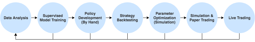
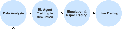
Luckily, there are solutions to many of the above problems. The bad news is, the solutions are not very effective. Let’s look a typical workflow for trading strategy development. It looks something like this:
-
Data Analysis: You perform exploratory data analysis to find trading opportunities. You may look at various charts, calculate data statistics, and so on. The output of this step is an “idea” for a trading strategy that should be validated.
-
Supervised Model Training: If necessary, you may train one or more supervised learning models to predict quantities of interest that are necessary for the strategy to work. For example, price prediction, quantity prediction, etc.
-
Policy Development: You then come up with a rule-based policy that determines what actions to take based on the current state of the market and the outputs of supervised models. Note that this policy may also have parameters, such as decision thresholds, that need to be optimized. This optimization is done later.
-
Strategy Backtesting: You use a simulator to test an initial version of the strategy against a set of historical data. The simulator can take things such as order book liquidity, network latencies, fees, etc into account. If the strategy performs reasonably well in backtesting, we can move on and do parameter optimization.
-
Parameter Optimization: You can now perform a search, for example a grid search, over possible values of strategy parameters like thresholds or coefficient, again using the simulator and a set of historical data. Here, overfitting to historical data is a big risk, and you must be careful about using proper validation and test sets.
-
Simulation & Paper Trading: Before the strategy goes live, simulation is done on new market data, in real-time. That’s called paper trading and helps prevent overfitting. Only if the strategy is successful in paper trading, it is deployed in a live environment.
-
Live Trading: The strategy is now running live on an exchange.
That’s a complex process. It may vary slightly depending on the firm or researcher, but something along those lines typically happens when new trading strategies are developed. Now, why do I think this process is not effective? There are a couple of reasons.
-
Iteration cycles are slow. Step 1-3 are largely based on intuition, and you don’t know if your strategy works until the optimization in step 4-5 is done, possibly forcing you to start from scratch. In fact, every step comes with the risk of failing and forcing you to start from scratch.
-
Simulation comes too late. You do not explicitly take into account environmental factors such as latencies, fees, and liquidity until step 4. Shouldn’t these things directly inform your strategy development or the parameters of your model?
-
Policies are developed independently from supervised models even though they interact closely. Supervised predictions are an input to the policy. Wouldn’t it make sense to jointly optimize them?
-
Policies are simple. They are limited to what humans can come up with.
-
Parameter optimization is inefficient. For example, let’s assume you are optimizing for a combination of profit and risk, and you want to find parameters that give you a high Sharpe Ratio. Instead of using an efficient gradient-based approach you are doing an inefficient grid search and hope that you’ll find something good (while not overfitting).
Let’s take a look at how a Reinforcement Learning approach can solve most of these problems.
Deep Reinforcement Learning for Trading
- Remember that the traditional Reinforcement Learning problem can be formulated as a Markov Decision Process (MDP). We have an agent acting in an environment. Each time step
- the agent receives as the input the current state
- , takes an action
- , and receives a reward
- and the next state
- . The agent chooses the action based on some policy
. It is our goal to find a policy that maximizes the cumulative reward
over some finite or infinite time horizon.


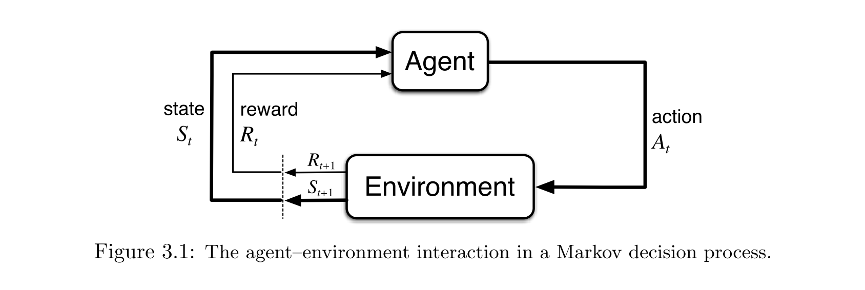
Let’s try to understand what these symbols correspond to in the trading setting.
Agent
Let’s start with the easy part. The agent is our trading agent. You can think of the agent as a human trader who opens the GUI of an exchange and makes trading decision based on the current state of the exchange and his or her account.
Environment
Here it gets a little hairy. The obvious answer would be that the exchange is our environment. But the important thing to note is that there are many other agents, both human and algorithmic market players, trading on the same exchange. Let’s assume for a moment that we are taking actions on a minutely scale (more on that below). We take some action, wait a minute, get a new state, take another action, and so on. When we observe a new state it will be the response of the market environment, which includes the response of the other agents. Thus, from the perspective of our agent, these agents are also part of the environment. They’re not something we can control.
However, by putting other agents together into some big complex environment we lose the ability to explicitly model them. For example, one can imagine that we could learn to reverse-engineer the algorithms and strategies that other traders are running and then learn to exploit them. Doing so would put us into a Multi-Agent Reinforcement Learning (MARL) problem setting, which is an active research area. I’ll talk more about that below. For simplicity, let’s just assume we don’t do this, and assume we’re interacting with a single complex environment that includes the behavior of all other agents.
State
In the case of trading on an exchange, we do not observe the complete state of the environment. For example, we don’t know about the other agents are in the environment, how many there are, what their account balances are, or what their open limit orders are. This means, we are dealing with a Partially Observable Markov Decision Process (POMDP). What the agent observes is not the actual state 


In our case, the observation at each timestep 
Time Scale
We need to decide what time scale we want to act on. Days? Hours? Minutes? Seconds? Milliseconds? Nanoseconds? Variables scales? All of these require different approaches. Someone buying an asset and holding it for several days, weeks or months is often making a long-term bet based on analysis, such as “Will Bitcoin be successful?”. Often, these decisions are driven by external events, news, or a fundamental understanding of the assets value or potential. Because such an analysis typically requires an understanding of how the world works, it can be difficult to automate using Machine Learning techniques. On the opposite end, we have High Frequency Trading (HFT) techniques, where decisions are based almost entirely on market microstructure signals. Decisions are made on nanosecond timescales and trading strategies use dedicated connections to exchanges and extremely fast but simple algorithms running of FPGA hardware. Another way to think about these two extremes is in term of “humanness”. The former requires a big picture view and an understanding of how the world works, human intuition and high-level analysis, while the latter is all about simple, but extremely fast, pattern matching.
Neural Networks are popular because, given a lot of data, they can learn more complex representations than algorithms such as Linear Regression or Naive Bayes. But Deep Neural Nets are also slow, relatively speaking. They can’t make predictions on nanosecond time scales and thus cannot compete with the speed of HFT algorithms. That’s why I think the sweet spot is somewhere in the middle of these two extremes. We want to act on a time scale where we can analyze data faster than a human possibly could, but where being smarter allows us to beat the “fast but simple” algorithms. My guess, and it really is just a guess, is that this corresponds to acting on timescales somewhere between a few milliseconds and a few minutes. Humans traders can act on these timescales as well, but not as quickly as algorithms. And they certainly cannot synthesize the same amount of information that an algorithm can in that same time period. That’s our advantage.
Another reason to act on relatively short timescales is that patterns in the data may be more apparent. For example, because most human traders look at the exact same (limited) graphical user interfaces which have pre-defined market signals (like the MACD signal that is built into many exchange GUIs), their actions are restricted to the information present in those signals, resulting in certain action patterns. Similarly, algorithms running in the market act based on certain patterns. Our hope is that Deep RL algorithms can pick up those patterns and exploit them.
Note that we could also act on variable time scales, based on some signal trigger. For example, we could decide to take an action whenever a large trade occurred in the market. Such as trigger-based agent would still roughly correspond to some time scale, depending on the frequency of the trigger event.
Action Space
In Reinforcement Learning, we make a distinction between discrete (finite) and continuous (infinite) action spaces. Depending on how complex we want our agent to be, we have a couple of choices here. The simplest approach would be to have three actions: Buy, Hold, and Sell. That works, but it limits us to placing market orders and to invest a deterministic amount of money at each step. The next level of complexity would be to let our agent learn how much money to invest, for example, based on the uncertainty of our model. That would put us into a continuous action space, as we need to decide on both the (discrete) action and the (continuous) quantity. An even more complex scenario arises when we want our agent to be able to place limit orders. In that case our agent must decide the level (price) and the quantity of the order, both of which are continuous quantities. It must also be able to cancel open orders that have not yet been matched.
Reward Function
This is another tricky one. There are several possible reward functions we can pick from. An obvious one would the Realized PnL (Profit and Loss). The agent receives a reward whenever it closes a position, e.g. when it sells an asset it has previously bought, or buys an asset it has previously borrowed. The net profit from that trade can be positive or negative. That’s the reward signal. As the agent maximizes the total cumulative reward, it learns to trade profitably. This reward function is technically correct and leads to the optimal policy in the limit. However, rewards are sparse because buy and sell actions are relatively rare compared to doing nothing. Hence, it requires the agent to learn without receiving frequent feedback.
An alternative with more frequent feedback would be the Unrealized PnL, which the net profit the agent would get if it were to close all of its positions immediately. For example, if the price went down after the agent placed a buy order, it would receive a negative reward even though it hasn’t sold yet. Because the Unrealized PnL may change at each time step, it gives the agent more frequent feedback signals. However, the direct feedback may also bias the agent towards short-term actions when used in conjunction with a decay factor.
Both of these reward functions naively optimize for profit. In reality, a trader may want to minimize risk. A strategy with a slightly lower return but significantly lower volatility is preferably over a highly volatile but only slightly more profitable strategy. Using the Sharpe Ratio is one simple way to take risk into account, but there are many others. We may also want to take into account something like Maximum Drawdown, described above. One can image a wide range of complex reward function that trade-off between profit and risk.
The Case for Reinforcement Learning
Now that we have an idea of how Reinforcement Learning can be used in trading, let’s understand why we want to use it over supervised techniques. Developing trading strategies using RL looks something like this. Much simpler, and more principled than the approach we saw in the previous section.
End-to-End Optimization of what we care about
In the traditional strategy development approach we must go through several steps, a pipeline, before we get to the metric we actually care about. For example, if we want to find a strategy with a maximum drawdown of 25%, we need to train supervised model, come up with a rule-based policy using the model, backtest the policy and optimize its hyperparameters, and finally assess its performance through simulation.
Reinforcement Learning allows for end-to-end optimization and maximizes (potentially delayed) rewards. By adding a term to the reward function, we can for example directly optimize for this drawdown, without needing to go through separate stages. For example, you could imagine giving a large negative reward whenever a drawdown of more than 25% happens, forcing the agent to look for a different policy. Of course, we can combine drawdown with many other metrics you care about. This is not only easier, but also a much more powerful model.
Learned Policies
Instead of needing to hand-code a rule-based policy, Reinforcement Learning directly learns a policy. There’s no need for us to specify rules and thresholds such as “buy when you are more than 75% sure that the market will move up”. That’s baked in the RL policy, which optimizes for the metric we care about. We’re removing a full step from the strategy development process! And because the policy can be parameterized by a complex model, such as a Deep Neural network, we can learn policies that are more complex and powerful than any rules a human trader could possibly come up with. And as we’ve seen above, the policies implicitly take into account metrics such as risk, if that’s something we’re optimizing for.
Trained directly in Simulation Environments
We needed separate backtesting and parameter optimization steps because it was difficult for our strategies to take into account environmental factors, such as order book liquidity, fee structures, latencies, and others, when using a supervised approach. It is not uncommon to come up with a strategy, only to find out much later that it does not work, perhaps because the latencies are too high and the market is moving too quickly so that you cannot get the trades you expected to get.
Because Reinforcement Learning agents are trained in a simulation, and that simulation can be as complex as you want, taking into account latencies, liquidity and fees, we don’t have this problem! Getting around environmental limitations is part of the optimization process. For example, if we simulate the latency in the Reinforcement Learning environment, and this results in the agent making a mistake, the agent will get a negative reward, forcing it to learn to work around the latencies.
We could take this a step further and simulate the response of the other agents in the same environment, to model impact of our own orders, for example. If the agent’s actions move the price in a simulation that’s based on historical data, we don’t know how the real market would have responded to this. Typically, simulators ignore this and assume that orders do not have market impact. However, by learning a model of the environment and performing rollouts using techniques like a Monte Carlo Tree Search (MCTS), we could take into account potential reactions of the market (other agents). By being smart about the data we collect from the live environment, we can continuously improve our model. There exists an interesting exploration/exploitation tradeoff here: Do we act optimally in the live environment to generate profits, or do we act suboptimally to gather interesting information that we can use to improve the model of our environment and other agents?
That’s a very powerful concept. By building an increasingly complex simulation environment that models the real world you can train very sophisticated agents that learn to take environment constraints into account.
Learning to adapt to market conditions
Intuitively, certain strategies and policies will work better in some market environments than others. For example, a strategy may work well in a bearish environment, but lose money in a bullish environment. Partly, this is due to the simplistic nature of the policy, which does not have a parameterization powerful enough to learn to adapt to changing market conditions.
Because RL agents are learning powerful policies parameterized by Neural Networks, they can also learn to adapt to various market conditions by seeing them in historical data, given that they are trained over a long time horizon and have sufficient memory. This allows them to be much more robust to changing markets. In facts, we can directly optimize them to become robust to changes in market conditions, by putting appropriate penalties into your reward function.
Ability to model other agents
A unique ability of Reinforcement Learning is that we can explicitly take into account other agents. So far we’ve always talked about “how the market reacts”, ignoring that the market is really just a group of agents and algorithms, just like us. However, if we explicitly modeled the other agents in the environment, our agent could learn to exploit their strategies. In essence, we are reformulating the problem from “market prediction” to “agent exploitation”. This is much more similar to what we are doing in multiplayer games, like DotA.
The Case for Trading Agent Research
My goal with this post is not only to give an introduction to Reinforcement Learning for Trading, but also to convince more researchers to take a look at the problem. Let’s take a look what makes Trading an interesting research problem.
Live Testing and Fast Iteration Cycle
When training Reinforcement Learning agents, it is often difficult or expensive to deploy them in the real world and get feedback. For example, if you trained an agent to play Starcraft 2, how would you let it play against a larger number of human players? Same for Chess, Poker, or any other game that is popular in the RL community. You would probably need to somehow enter a tournament and let your agent play there.
Trading agents have characteristics very similar to those for multiplayer games. But you can easily test them live! You can deploy your agent on an exchange through their API and immediately get real-world market feedback. If your agent does not generalize and loses money you know that you have probably overfit to the training data. In other words, the iteration cycle can be extremely fast.
Large Multiplayer Environments
The trading environment is essentially a multiplayer game with thousands of agents acting simultaneously. This is an active research area. We are now making progress at multiplayer games such as Poker, Dota2, and others, and many of the same techniques will apply here. In fact, the trading problem is a much more difficult one due to the sheer number of simultaneous agents who can leave or join the game at any time. Understanding how to build models of other agents is only one possible direction one can go into. As mentioned earlier, one could choose to perform actions in a live environment with the goal maximizing the information gain with respect to kind policies the other agents may be following.
Learning to Exploit other Agents & Manipulate the Market
Closely related is the question of whether we can learn to exploit other agents acting in the environment. For example, if we knew exactly what algorithms were running in the market we can trick them into taking actions they should not take and profit from their mistakes. This also applies to human traders, who typically act based on a combination of well-known market signals, such as exponential moving averages or order book pressures.
Disclaimer: Don’t allow your agent to do anything illegal! Do comply with all applicable laws in your jurisdiction. And finally, past performance is no guarantee of future results.
Sparse Rewards & Exploration
Trading agents typically receive sparse rewards from the market. Most of the time you will do nothing. Buy and sell actions typically account for a tiny fraction of all actions you take. Naively applying “reward-hungry” Reinforcement Learning algorithms will fail. This opens up the possibility for new algorithms and techniques, especially model-based ones, that can efficiently deal with sparse rewards.
A similar argument can be made for exploration. Many of today’s standard algorithms, such as DQN or A3C, use a very naive approach to exploration, basically adding random noise to the policy. However, in the trading case, most states in the environment are bad, and there are only a few good ones. A naive random approach to exploration will almost never stumble upon those good state-actions pairs. A new approach is necessary here.
Multi-Agent Self-Play
Similar to how self-play is applied to two-player games such as Chess or Go, one could apply self-play techniques to a multiplayer environment. For example, you could imagine simultaneously training a large number of competing agents, and investigate whether the resulting market dynamic somehow resembles the dynamics found in the real world. You could also mix the types of agents you are training, from different RL algorithms, the evolution-based ones, and deterministic ones. One could also use the real-world market data as a supervised feedback signal to “force” the agents in the simulation to collectively behave like the real world.
Continuous Time
Because markets change on micro- to milliseconds times scales, the trading domain is a good approximation of a continuous time domain. In our example above we’ve fixed a time period and made that decision for the agent. However, you could imagine making this part of the agent training. Thus, the agent would not only decide what actions to take, but also when to take an action. Again, this is an active research area useful for many other domains, including robotics.
Nonstationary, Lifelong Learning, and Catastrophic Forgetting
The trading environment is inherently nonstationary. Market conditions change and other agent join, leave, and constantly change their strategies. Can we train agents that learn to automatically adjust to changing market conditions, without “forgetting” what they have learned before? For example, can an agent successfully transition from a bear to a bull market and then back to a bear market, without needing to be re-trained? Can an agent adjust to other agent joining and learning to exploit them automatically?
Transfer Learning and Auxiliary Tasks
Training Reinforcement Learning from scratch in complex domains can take a very long time because they not only need to learn to make good decisions, but they also need to learn the “rules of the game”. There are many ways to speed up the training of Reinforcement Learning agents, including transfer learning, and using auxiliary tasks. For example, we could imagine pre-training an agent with an expert policy, or adding auxiliary tasks, such as price prediction, to the agent’s training objective, to speed up the learning.
Conclusion
The goal was to give an introduction to Reinforcement Learning based trading agents, make an argument for why they are superior to current trading strategy development models, and make an argument for why I believe more researcher should be working on this. I hope I achieved some this in this post. Please let me know in the comments what you think, and feel free to get in touch to ask questions.
Thanks for reading all the way to the end :)