Getting Started With MapD, Part 1： Docker Install and Loading Data

It’s been nearly five years since I wrote about Getting Started with Hadoop for big data. In those years, there have been incremental improvements in columnar file formats and dramatic computation speed improvements with Apache Spark, but I still wouldn’t call the Hadoop ecosystem convenient for actual data analysis. During this same time period, thanks to NVIDIA and their CUDA library for general-purpose calculations on GPUs, graphics cards went from enabling visuals on a computer to enabling massively-parallel calculations as well.

Building upon CUDA is MapD, an analytics platform that allows for super-fast SQL queries and interactive visualizations. In this blog post, I’ll show how to use Docker to install MapD Community Edition and load hourly electricity demand data to analyze.

Installing MapD CE using Docker/nvidia-docker

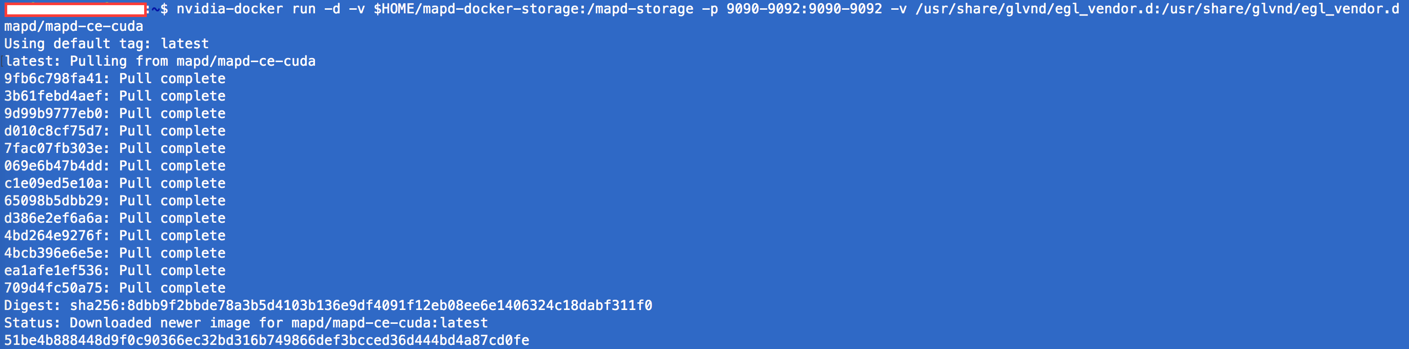
While CUDA makes it possible to do calculations on GPUs, I wouldn’t go as far as to say it is easy, including just getting everything installed! Luckily, there is Docker and nvidia-docker, which provide all-in-one containers with all necessary drivers and libraries installed to build upon. MapD provides instructions for installing MapD CE using nvidia-docker, with the main installation command as follows:

|1
2
3
4
5
|##nvidia-docker version 2
docker run --runtime=nvidia \
-v $HOME/mapd-docker-storage:/mapd-storage \
-p 9090-9092:9090-9092 \
mapd/mapd-ce-cuda

When you kickoff this command (I’m using a ssh terminal into a remote Ubuntu desktop), Docker will download all the required images from the mapd/mapd-ce-cudarepository and start a background process for the MapD database and the Immerse visualization interface/web server:

Once all of the images are downloaded, you can find the container that was created using docker container ls, then run docker exec -it <container id> bash to start the container and drop you into a Bash shell (on the container). From this point, MapD Community Edition will be running!

Loading Data Using the Immerse Interface

Once the Bash shell opens in the terminal, you can now interact with MapD via the Docker container. However, for beginning exploration, it’s much simpler to use the Immerse Web Interface at localhost:9092:

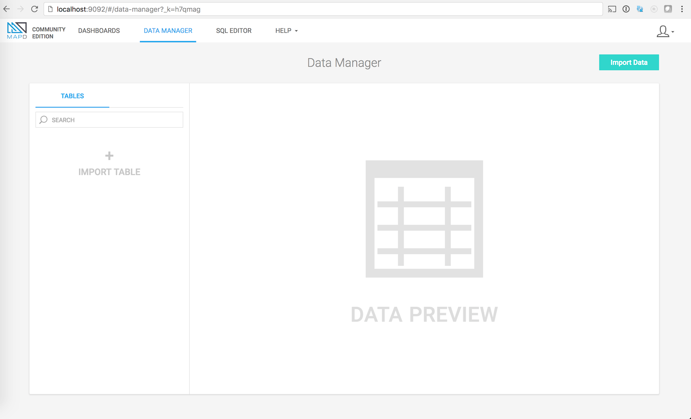
Uploading data via the Data Manager interface is reasonably performant for smaller files; a test file with four columns and million or so rows loaded in a few seconds (dependent on your upload speed, obviously):

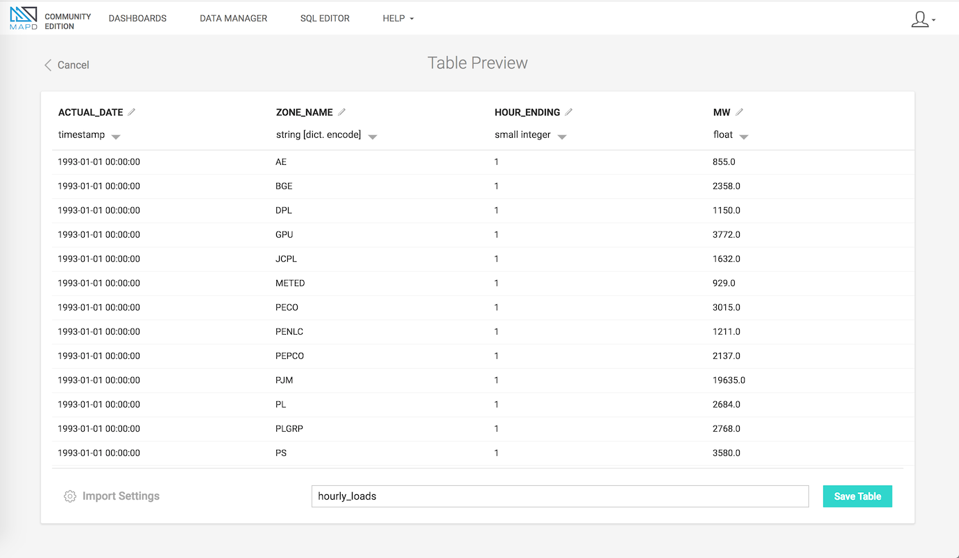
Edit the column names and types if you want (the CSV reader gets it right for me most of the time). Then, once the ‘Save Table’ button is clicked, MapD will import the CSV data into a columnar binary format, so that the GPU can operate directly on the data rather than reading from the CSV each query.

Loading Data Using the Command Line

While browser GUIs are great for some things, I’m still very much a command-line guy, at least for things like loading data. MapD provides the mapdql interface to load data and query, very much like psql for Postgres and other databases. To load my 4.9 million * 4 column dataset, I used the following commands:

|1
2
3
4
5
6
7
8
9
10
11
12
13
14
15
16
17
18
|$ docker container ls
CONTAINER ID IMAGE COMMAND CREATED STATUS PORTS NAMES
51be4b888448 mapd/mapd-ce-cuda "/bin/sh -c '/mapd/s…" 44 hours ago Up 44 hours 0.0.0.0:9090-9092->9090-9092/tcp nifty_heisenberg

$ docker exec -it 51be4b888448 bash
root@1f64b2dcc316:/mapd# bin/mapdql
Password: <default is "HyperInteractive">
User mapd connected to database mapd

mapdql> create table hourly_loads(
..> ACTUAL_DATE DATE,
..> ZONE_NAME TEXT,
..> HOUR_ENDING SMALLINT,
..> MW FLOAT);

mapdql> copy hourly_loads from 'hourly_loads.csv';
Result
Loaded: 4898472 recs, Rejected: 0 recs in 0.923000 secs

The DDL for MapD seems pretty much the same as every other database language. First you define a table’s columns and their types, then you can use the copy command to load data from a CSV. The statement that prints upon success begins to give an indication of the speed MapD provides, loading nearly 5 million records in less than a second.

Simplistic Query Performance

Up this point, I’ve intentionally not described the data I uploaded into MapD; in my next post, I’ll cover the dataset I’m using and how I converted the data from Excel spreadsheets into a CSV. But before ending this post, I wanted to show a brief summary of the performance of MapD:

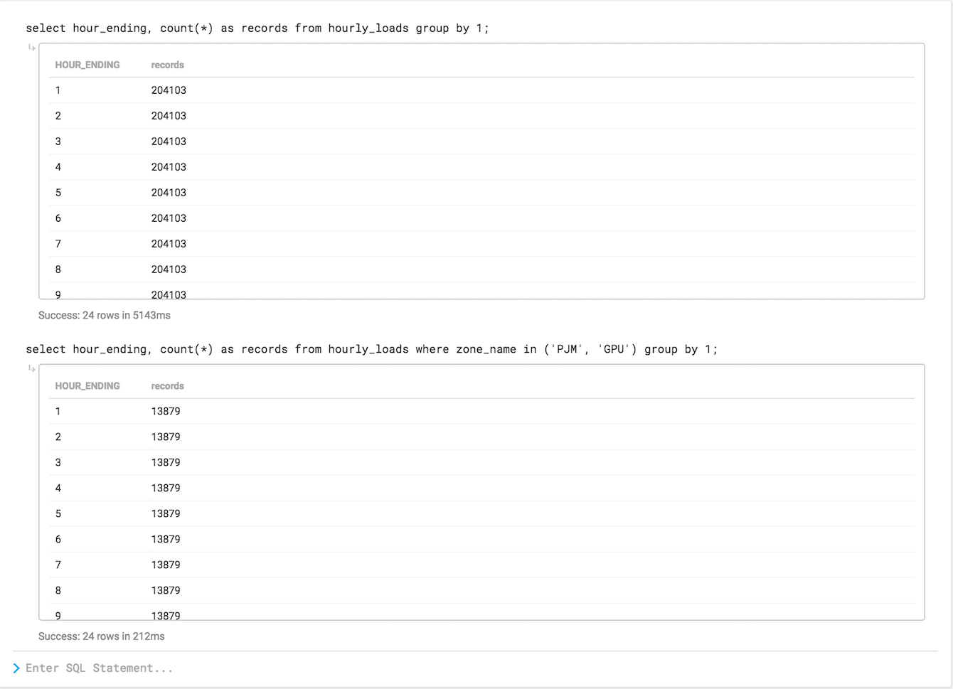
The first query shows a simple record count by the hour_ending dimension in my table, something you might run if you weren’t too familiar with the table. You’ll notice that running this group by across the 5 million row dataset took 5143ms, which isn’t so fast. What’s going on?

Because this is the first query from a cold start, MapD needs to load data into GPU RAM. So while the first query takes a few seconds, the second query displays a warmed-up level of performance: 212ms to scan 5 million rows, filter by a few values of the zone_name column, then grouping by hour_ending. For reference, a human blink takes 100-400 ms, so this second query quite literally finished in the blink of an eye…

Dashboards, Streaming Data and more…

This first blog post just scratched the surface on what is possible using just the Community Edition of MapD. In future blog posts, I will provide the code to create the dataset, do some basic descriptive statistics, and even do some analysis and dashboarding of historical electricity demand.

Update, 2/1/2018 4:49 p.m.

Per Todd Mostak from MapD, the second query would likely even run faster than 212ms, had I run it again: