Normal Distributions

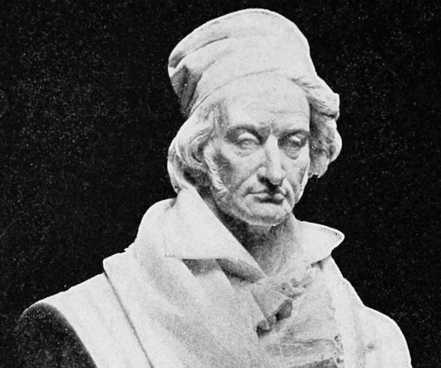
I review — and provide derivations for — some basic properties of Normal distributions. Topics currently covered: (i) Their normalization, (ii) Samples from a univariate Normal, (iii) Multivariate Normal distributions, (iv) Central limit theorem.

Introduction

This post contains a running list of properties (with derivations) relating to Normal (Gaussian) distributions. Normal distributions are important for two principal reasons: Their significance a la the central limit theorem and their appearance in saddle point approximations to more general integrals. As usual, the results here assume familiarity with calculus and linear algebra.

Pictured at right is an image of Gauss — “Few, but ripe.”

Normalization

Consider the integral\begin{eqnarray} \tag{1}I = \int_{-\infty}^{\infty} e^{-x^2} dx.\end{eqnarray}To evaluate, consider the value of $I^2$. This is\begin{eqnarray}\tag{2}I^2 &=& \int_{-\infty}^{\infty} e^{-x^2} dx \int_{-\infty}^{\infty} e^{-y^2} dy \&=& \int_0^{\infty} e^{-r^2} 2 \pi r dr = -\pi e^{-r^2} \vert_0^{\infty} = \pi.\end{eqnarray}Here, I have used the usual trick of transforming the integral over the plane to one over polar $(r, \theta)$ coordinates. The result above gives the normalization for the Normal distribution.

Samples from a univariate normal

Suppose $N$ independent samples are taken from a Normal distribution. The sample mean is defined as $\hat{\mu} = \frac{1}{N}\sum x_i$ and the sample variance as $\hat{S}^2 \equiv \frac{1}{N-1} \sum (x_i – \hat{\mu})^2$. These two statistics are independent. Further, the former is Normal distributed with variance $\sigma^2/N$ and the latter is proportional to a $\chi_{N-1}^2.$

Proof: * Let the sample be $\textbf{x} = (x_1, x_2, \ldots, x_N)$. Then the mean can be written as $\textbf{x} \cdot \textbf{1}/N$, the projection of $\textbf{x}$ along $\textbf{1}/N$. Similarly, the sample variance can be expressed as the squared length of $\textbf{x} – (\textbf{x} \cdot \textbf{1} / N)\textbf{1} = \textbf{x} – (\textbf{x} \cdot \textbf{1} / \sqrt{N})\textbf{1}/\sqrt{N}$, which is the squared length of $\textbf{x}$ projected into the space orthogonal to $\textbf{1}$. The independence of the ${x_i}$ implies that these two variables are themselves independent, the former Normal and the latter $\chi^2_{N-1}.$
The result above implies that the weight for sample $\textbf{x}$ can be written as\begin{eqnarray} \tag{3}p(\textbf{x} \vert \mu, \sigma^2) = \frac{1}{(2 \pi \sigma^2)^{N/2}} \exp\left [ – \frac{1}{2 \sigma^2}\left ( – N (\hat{\mu} – \mu)^2 – (N-1)S^2\right) \right].\end{eqnarray}