||
This week I’m going to talk about Voronoi diagrams. These constructions are really pretty, and simple to explain.

Imagine I’m in a desert, and there are two wells where I can obtain water. If I want to go to the nearest well, which well do I visit? Clearly, it depends one where I am standing. It’s possible to draw a line dividing the desert. To the ‘left’ of the line, it’s nearer to go to the well on the well on the ‘left’, to the ‘right’ of the line, it’s closer to go to the well on the ‘right’.
The line dividing which well is nearer is a straight line. Also, if I had infinitely small feet, and I stood anywhere on this line, I’d be equidistant from both of the wells.
It’s easy to see that dividing line bisects the perpendicular straight line connecting both wells. Additionally, if I drew two circles of any same (arbitrary) radius greater than half the distance between the wells, then they would overlap on this line.
What happens if I add a third well? Or a fourth? We now get regions like these. Each of the boundaries’ partitions off the space for which well is nearer. These are Voroni diagrams (sometimes called Voronoi Tesesellations, Dirichlet Tessellations, or Thiessen polygons). They are named after Georgy Feodosevich Voronoi, a Ukrainian mathematician, who died in 1908. (To celebrate the centenary of Voronoi, Ukraine released a two-hryvnia coin for him).
Rather than simply showing just the boundaries, we can shade each region with a colour representing all the pixels that are closest to each node. Here are some examples. The regions tessellate perfectly, and are easy to decode.
Here’s a couple of animated versions where some of the points are moving. It’s mesmerizing to watch how the regions morph as their nodes pass by each other and the regions representing the nearest points change in geometery.
Generating Voronoi Diagrams
There are many ways to generate Voronoi diagrams. The easiest to understand is a simple brute force approach: For each pixel we care about, simply calculate the distance from each of the nodes. Whichever of these distances is the shortest, colour the pixel with that colour. Done!
This brute force approach is not very efficient, and the code ends up calculating distances for nodes that are clearly not in the running.
Another possible strategy is a kind of flood fill: We can generate circles of ever-increasing radii from each node until they touch. (Or you could think about them as crystals growing from nucleation sites). Here’s a couple of animations of this:
An analogous way to think about these growing circles is to imagine them as cones in 3D extruding out of the plane.
|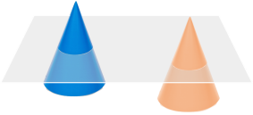 |Imagine a cone with apex at each node, and then these cones slowly being pushed through a plane. As they pass through, they generate circles. These circles continue to grow until they hit the edges of other cones.This gives hints to how Voronoi diagrams can be generated using a 3D graphics technique; using cones plotted into a depth buffer. 3D Graphics cards use a Z-buffer (a value for each pixel of the display) to determine which is the ‘nearest’ pixel to the viewer to perform hidden surface removal (thus it only renders the pixel for the object nearest). |
This gives hints to how Voronoi diagrams can be generated using a 3D graphics technique; using cones plotted into a depth buffer. 3D Graphics cards use a Z-buffer (a value for each pixel of the display) to determine which is the ‘nearest’ pixel to the viewer to perform hidden surface removal (thus it only renders the pixel for the object nearest).
Images: Matt Keeter
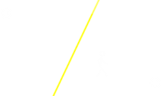
There’s another interesting algorithm named after Steven Fortune, who published it in a paper in 1986. Fortune’s algorithm sweeps a straight line across the region. In the diagram to the left, points to the right of the sweeping red straight line have not been considered yet. The sweep line drags behind it a ‘beach line’ which is a curve composed of parabolas. The beach line divides regions where it is known which nodes is the closest, and those that it has yet to be determined. For each point left of the sweep line, one can define a parabola of points equidistant from that point and from the sweep line; the beach line is the boundary of the union of these parabolas. As the sweep line progresses, the vertices of the beach line, at which two parabolas cross, trace out the edges of the Voronoi diagram. The beach line progresses by keeping each parabola base exactly half way between the points initially swept over with the sweep line, and the new position of the sweep line. Here’s a link to more details on Fortune’s Algorithm.
Interactive demo
|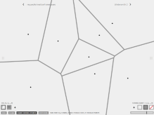 |If you want to experiment with creating these diagrams, I highly recommend playing with the application on this page Voronoi Painter written by Johan Nordberg (To make it easy to see what is going on, press [P] to toggle display of the points). It’s a pretty fun toy to play with.|
Applications of Voronoi Tessellations
If you are the pilot of an aircraft, at any time, you might want to know which is the nearest available airport you could land at if an inflight emergency occured. Here’s an interactive demo based on major airports.
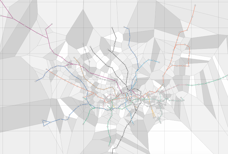
Here’s a fabulous map of the Tube Stations on the London Underground. It shows which is the nearest tube station to any location.
A noteworthy application appeared in John Snow’s
Snow then considered the sources of drinking water, pumps distributed throughout the city, and drew a line labeled “Boundary of equal distance between Broad Street Pump and other Pumps” which indicated the Broad Street Pump’s Voronoi cell.
This map supported Snow’s hypothesis that the cholera deaths were associated with contaminated water, in this case, from the Broad Street Pump. Snow recommended that the pump handle be removed, after which action the cholera outbreak quickly ended. Snow’s work helped develop the modern field of epidemiology, and this map has been called “The most famous 19th century disease map”.
Voronoi maps have uses in Archeology and Anthropology to identify regions under the influence of different clans, and in Biology to compare plant and animal competitions. In Geography and Marketing they can be used to map regions based on sparse samples.
Some of the earliest recorded uses of Voronoi diagrams are in Astronomy. In 1744 Descartes was using them to describe the influences of regions of stars and galaxies.
If your job was to build a nuclear waste storage depot and a crieterion was that it had to be as far away as possible from any city, you can see how it must be located on a Voronoi edge. Maybe you have to fly your spy plane across a country and want to select a path that is the furthest distance away from every radar station to minimize the chance that you are detected. A maximally clear path will follow the lines edges of a Voronoi tessellation. Do you need to traverse a battlefield keeping a maximal distance for a group of snipers?
A less severe application of this technique could be used by autonomous vehicles and drones to plot paths through congested spaces so as to keep them as far away as possible from all detected obstacles (see left).
As we will see next, Voronoi tessellations have applications for making efficient triangular meshes, which are incredibly useful for finite element anlysis, computer graphics, video games, and modeling …
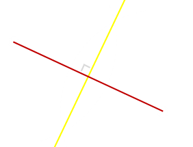
|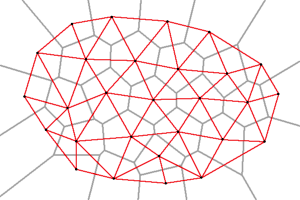 |If you create a dual graph of a Voronoi diagram (connect each node to every other node that shares an edge), you end up with a graph that is a Dalaunay Triangulation (a construct just as interesting as Voronoi tessleations and will sure to be a feature of a future blog posting).In the diagram to the left, the red lines represent a Delaunay Triangulation.Delaunay triangulations are leveraged heavily in many applications, especially computer graphics, as they are ways to break up regions into triangles. 3D graphics cards are optimized to render triangles very efficiently.|
In the diagram to the left, the red lines represent a Delaunay Triangulation.
Three points make up a triangle, and there is only one way this can happen. As soon as a polygon has more than three vertices, however, if you have to break this shape into a plurality of triangles, there are multiples ways this can happen.
For example, look at this quadrilateral below. If we had to break this up into two triangles, there are two ways:

Which is the ‘better’ way (for graphics). A Russian mathematician (and mountain climber), Boris Delaunay described a determinitic criterion for identifying how triangular meshes should be constructed, and the ‘best’ way to break up larger polygons into triangles. (Delaunay is also credited as being the organizer of the first mathematical olympiad for high school students in the Soviet Union).
His criteria is based on a circular test, and the goal is to minimze the occurence of sliver triangles (triangles with one or two extremely accute angles, which are undesirable in interpolation and rendering).

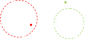
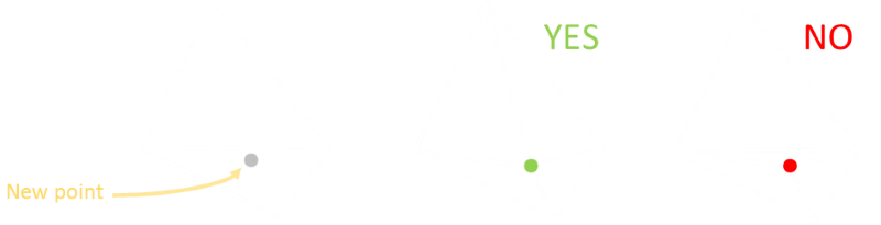
It’s a pretty simple test: draw a circle through the three vertices of any triangle on the grid. If the grid meets the Delaunay test, there should be no additional vertex inside the circle. In the quaderlateral below, the triangulation on the right passes this test, the one on the left does not. Therefore, the correct way to triangulate this is the way on the right.
Delaunay triangulations maximize the minimum angle of all the angles of the triangles in the triangulation.
In addition to maximizing the minimum angle in each triangle, here are some other properties of Delaunay meshes:
-
The vertices make up a convex hull (the same shape you’d get if you put an elastic band around the points). For more information about convex hulls, check out this article.
-
A Delaunay triangulation maximizes the minimum angle. Compared to any other triangulation of the points, the smallest angle in the Delaunay triangulation is at least as large as the smallest angle in any other. However, the Delaunay triangulation does not necessarily minimize the maximum angle. The Delaunay triangulation also does not necessarily minimize the length of the edges.
-
If a circle passing through two vertices doesn’t contain any other, then the segment connecting the two vertices is an edge of a Delaunay triangulation.
Flipping
Note: Just because a certain quadrilateral is broken into two triangles a certain way, it does not mean this division will always be there. As more vertices are added, this line can flip. Each time a new vertex is added, the test needs to be applied to see if it is still valid.
(This cascading flipping is one of the algorithms that can be used to generate a Delaunay mesh, but it’s not the most efficient).
Trying it out
Here’s nice little page that allows you to experinent and interact with the creation of Delaunay Meshes.
You can find a complete list of all the articles here. Click here to receive email alerts on new articles.