In this blog we will engineer a new feature to go into our model. So far we have predominantly been using localised features – information about pixels that are located nearby the pixel whose brightness we are predicting. In this blog we will consider the structure of a document, and use that to improve our model.

The image consists of multiple lines of text, arranged into one or more paragraphs with multiple sentences in each paragraph.

If we get our ducks in a row, we can use the fact that the text (like our metaphorical ducks) is arranged into lines, and that there are gaps between those lines of text. In particular, if we can find the gaps between the lines, we can ensure that the predicted value within those gaps is always the background colour.
Let’s look at the horizontal profile of a sample input image:

The rows with low brightness show where text occurs at regular intervals. But the absolute level of the row brightness varies, according to the noise and stains, so much that sometimes the gaps between the lines of text are darker than the rows in which text occurs. This will make it more difficult to determine which rows are which.
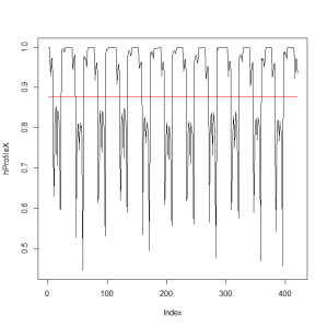
But what if we used the predicted images from our stacked model from the last blog as the inputs to this predictor?

Now it’s much easier to find the gaps between the lines of text. To do this we need estimate three parameters:
-
cycle length: the number of rows from one line of text to the next line of text
-
gap length: the height of the gap between lines of text
-
starting location of the first cycle
The constraints that we can use for determining these parameters are:
-
cycle length is a positive number
-
gap length is a positive number
-
gap length is less than cycle length
-
gap rows are white
-
most letters (e.g. weruioaszxcvnm) are short and these letters are located in the darkest rows, which we will call the “core rows”
-
some letters are taller (e.g. tdfhklb) and create slightly darker rows above the core rows
-
some letters are taller (e.g. qypgj) and create slightly darker rows below the core rows
-
if we cluster the values, the darker cluster contains the core of the letters (the core rows), but these rows may be lighter when a paragraph starts or ends
-
the in-between valued rows next to the white rows are possibly where the taller letters are located and their darkness will vary according to the number of tall letters
Let’s start by clustering the row brightnesses, and checking where the rows switch from one cluster to another, and using this to estimate cycle length.

Next we will estimate the starting location of the first cycle. But before we do that, we need to define the “start” of the cycle. Let’s define the cycle as starting at the row in which the first letter starts. That would be the first non-white row before the first core rows.
cycleStarts = starts[1]while (hProfileX[cycleStarts] < 0.99)cycleStarts = cycleStarts – 1
The first cycle starts at row 3.
To estimate the gap length, we should measure the number of white rows before each cycle starts.
The gaps are (13, 12, 17, 13, 12, 11, 12, 18, 12, 12). The two outliers occur after rows of text that do not contain any of the characters (q, y, p, g, j). After removing these two outliers, the gaps do not exceed 13 rows. So we can write code to allow for this as follows:
This gives us a gap length estimate of 13.125 and completes our line location model for this image. The quick way to use this model is to white out the gap rows. A more complex model could use the newly estimated row types (core, gap, other) as predictors.
The script above would clean up any minor image blemishes that exist between the lines of text.
Like this:
Like Loading…
Related