TIME SERIES ANALYSIS
Loosely speaking, a time series describes the behavior of a variable with time. For example a company’s daily closing stock prices. Our major interest lies in forecasting this variable or the stock price in our case in the future. We try to develop various statistical and machine learning models to fit the data, capture the patterns and forecast the variable well in the future.
In this article, we will try traditional models like ARIMA, popular machine learning algorithms like Random Forest and deep learning algorithms like LSTM.
Tutorial link (you can download the data from this repository)
https://github.com/DhruvilKarani/Time-Series-analysis/blob/master/Stock%20Price%20Prediction%20using%20ML%20and%20DL-Final.ipynb
The data looks something like this –
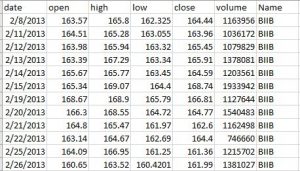
Now let’s explore the models.
ARIMA (Auto-Regressive Integrated Moving Average)
Before we actually dive into the model, let’s see if the data is in it’s the best form for our model.
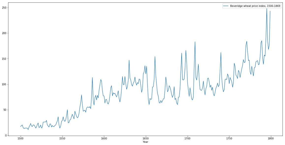
Clearly, we see there is an upwards trend. When we analyze a time series, we want it to be stationary, meaning the mean and variance should be constant along the time series. Why? This is because it is useful to analyze such a series from a statistical point of view. Like in our case, usually there exists a trend. To make a time series stationary, a common way is to *difference *it
I.e. a series having [a,b,c,d] is transformed to [b-a,c-b,d-c].
A differenced time series looks something like this –
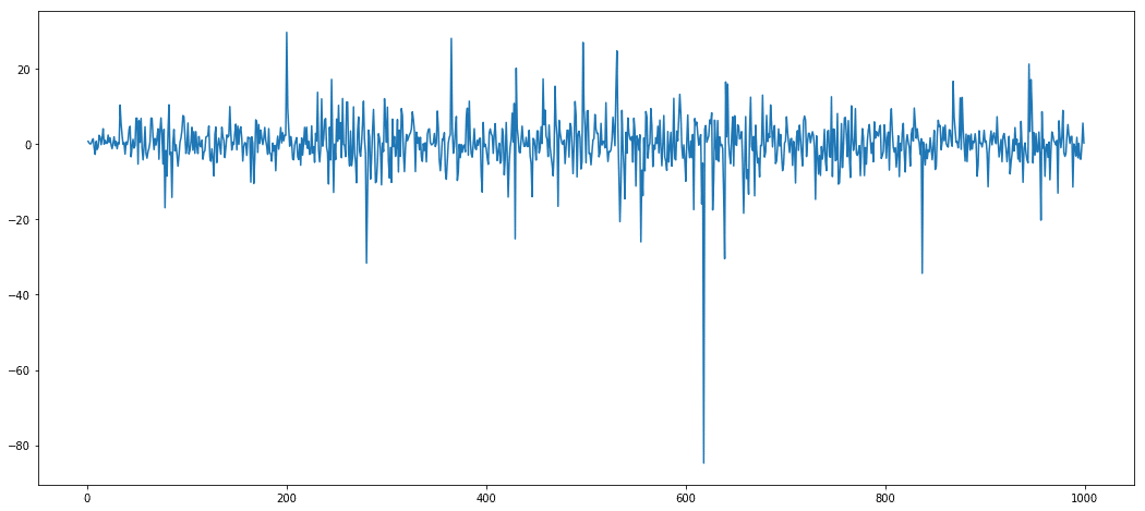
The mean and variance looks almost constant, except for a few outliers. Such a differenced time series is suitable for modelling.
OK! We know something about how our data should look like. But what exactly is ARIMA?
Let’s break it down into 3 terms
AR – This term indicates the number of auto-regressive terms (p) in the model. Intuitively, it denotes the number of previous time steps the current value of our variable depends on. For example, at time T, our variable Xt depends on Xt-1 and Xt-2, linearly. In this case, we have 2 AR terms and hence our p parameter=2
**I **– As stated earlier, to make our time series stationary, we have to difference it. Depending on the data, we difference it once or multiple times (usually once or twice). The number of times we do it is denoted by d.
**MA **– This term is a measure of the average over multiple time periods we take into account. For example, to calculate the value of our variable at the current time step, if we take an average over previous 2 timesteps, the number of MA terms, denoted by q=2
Specifying the parameters (p,d,q) will specify our model completely. But how do we select these parameters?
We use something called ACF (Autocorrelation plot) and PACF(Partial autocorrelation plot) for this purpose. Let’s get an intuition of what autocorrelation and partial autocorrelation mean.
We know that for 2 variables X and Y, correlation denotes how the two variables behave with each other. Highly positive correlation denotes that X increases with Y. Highly negative correlation denotes that X decreases with Y. So what is autocorrelation?
In a time series, it denotes the variance of the predicted variable at a particular time step with its previous time steps. Mathematically,

Where X’ is the mean, k is the lag (number of time steps we look back. k=1 means t-1), N is the total number of points. C is the autocovariance. For a stationary time series, c does not depend on t. It only depends on k or the lag.
Partial autocorrelation is a bit tricky concept. Just get an intuition for now. Consider an example – We have the following data – body fat level (F), triceps measurement (Tr) and thigh circumference (Th). We want to measure the correlation between F and Tr but we also don’t want thigh circumference or Th to play any role. So what do we do? We try to remove linearity from F and Tr introduced by Th. Let F’ be the fat levels predicted by Th, linearly. Similarly, let Tr’ be triceps measurement as predicted by Th, linearly.
The residuals for fat levels is given by F-F’ and for tricep measurement is given by Tr-Tr’. Partial correlation is the correlation measured between these residuals.
In our case the
Next, we answer two important questions
What suggests AR terms in a model?
-
ACF shows a decay
-
PACF cuts off quickly
What suggests MA terms in a model?
-
ACF cuts off sharply
-
PACF decays gradually
In our case, the ACF looks something like
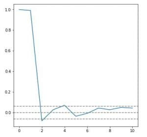
From lag 0 it decays gradually. The top and bottom grey dashed lines show the significance level. Between these levels, the autocorrelation is attributed to noise and not some actual relation. Therefore q=0
PACF looks like
It cuts off quickly, unlike the gradual decay in ACF. Lag 1 is significantly high, indicating the presence of 1 AR term. Therefore p=1.
So now we have specified our model. Let’s fir our ARIMA(p=1,d=1,q=0) model. Follow the tutorial to implement the model. Results look something like –
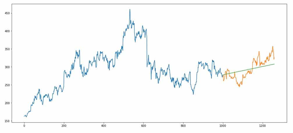
Blue portion is the data on which the model is fitted. Orange is the holdout/validation set. Green is our model’s performance. Note that we only need the predicted variable for ARIMA. Nothing else.
The mean squared error for our model turns out to be 439.38.
Machine and Deep learning algorithms
To see if machine learning and deep learning algorithms work well on our data, we test two algorithms – Random Forest and LSTM. The data is the same except for that we use all the features and not just the predicted variable. We do some basic feature engineering like extracting the month, day and year.
Deep Learning Model – LSTM
LSTM or long short-term memory network is a variation of the standard vanilla RNN (Recurrerent Neural Networks). RNNs, many times tend to suffer through a problem of vanishing/exploding gradients. This means that the gradient values become too large or too small, causing problems in updating the weights of RNN. LSTMs are improvised versions of RNN that solve this problem through the use of gates. For a detailed explanation, I highly recommend this video – https://youtu.be/8HyCNIVRbSU
In our case, we use Keras framework to train an LSTM.
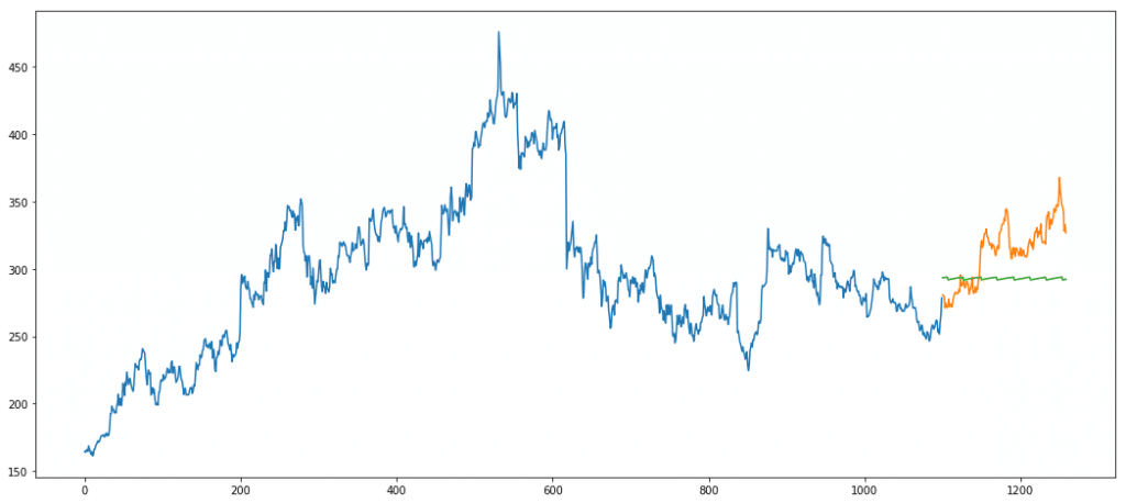
Error = 895.06
As we can see, LSTM performs really poorly on our data. Main reason is the lack of data. We train only on 1000 data points. This is really less for a deep neural network. This is a classic example where neural nets don’t always outperform traditional algorithms.
Random Forest
Random forest is a tree bases supervised machine learning algorithm. It builds short weak tree learners by randomly sampling features to split the data on. This ensures features getting adequate representation in the model unlike the greedy approach classical decision trees take.
Suppose we train 10 trees. For a data point, each tree outputs its own y value. In a regression problem the average of these 10 trees is taken as the final value for the data point. In classification, majority vote is the final call.
Using grid search we set the appropriate parameters. Our final predictions look something like
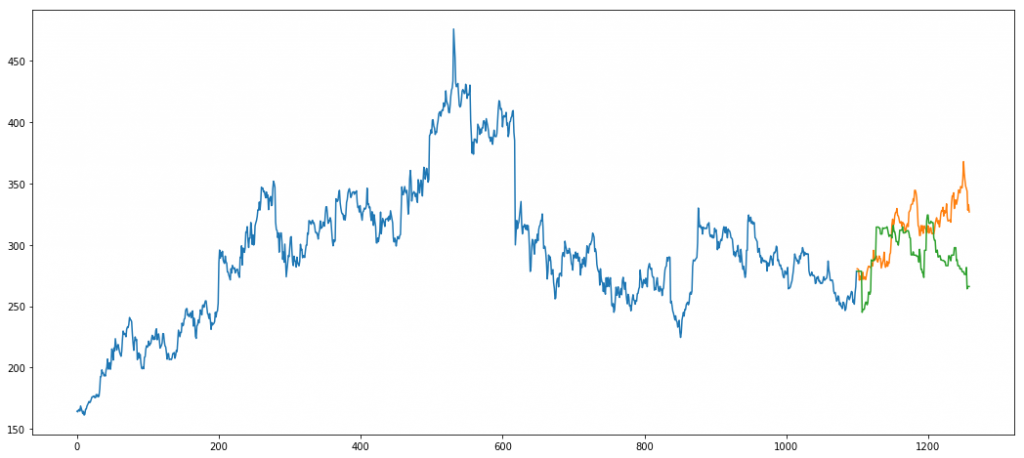
Error = 1157.91
If you notice carefully, our holdout set does not follow the peaks that our train set follows. The model fails to predict the same as it has learned to predict peaks like the ones in blue. Such an unexpected shift in trend is not captured by models.