By Nathalie Jeans.

The first thing people think of when they hear the term “Machine Learning” goes a little something like the Matrix. All around, there are computers taking over the world, let alone the human race. And maybe — just maybe — they’re making some music or creating some art on the side. In any case, people generally just want nothing to do with it.
What if I told you those people don’t even know what machine learning and things like backpropagation really are? Just hear me out. Then you can go back to worrying about the robot-led apocalypse that’s supposed to happen next Friday.
Deep Learning: Neural Networks, Weights, and Biases
A neural network is just a really complicated machine: you have an input, you put it through the machine, and you get something that comes out. There are multiple tasks that make up this machine so that you get what you want in the end. You can also adjust each of the tasks that are part of this process so you have the best-working, most accurate result at the end. In a neural network, the ‘tasks’ are hidden layers, while the adjustment of the tasks’ performance are called weights. This determines how each of the nodes within the hidden layers are considered which affects the result of the final output. The principle of machine learning states that the optimal final output can be obtained by adjusting the tasks through inputting larger amounts of datasets, like trial and error.
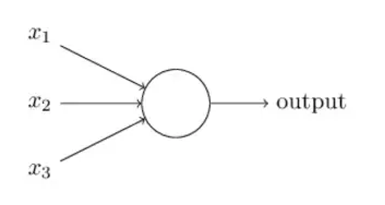
Let X1, X2, and X3 represent the inputs, and O represent the output. There are two different ways to compute this:
-
Take the sum of the inputs:O = X1 + X2 + X3. This process, while taking into account each of the inputs, does not account for how importantof each of them. You can’t tell how one of the inputs affects the other — only how they individually affect the result.
-
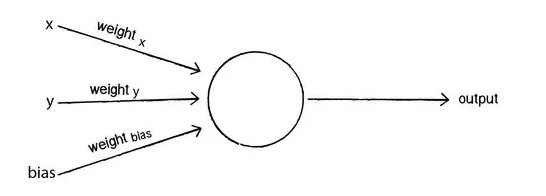
Apply a linear function operation:O = (X1*X2) + X3. This may seem familiar, and that’s because it’s in the form of a linear function y = mx + b (How well do you remember 8th grade math?). While X1 is the input, X2 would be the weight, and X3 is the bias. What this means is X2, because it is multiplied by X1, determines the importance of X1. The closer X2 is to 0, the less it affects the output. There is also the possibility that O = X3 if X1 or X2 = 0. In this case, X3 is the bias: it considers how much this output will be activated regardless of the input.
So, the result of your output is:
-
Output is 0 if {weight * X + b ≤ 0}
-
Output is 1 if {weight * X + b > 0}
-
Output is 1 if {(weight of X)* X + (weight of Y)*Y + b > 0}
-
Output is otherwise equal to 0
The values are of the output are discrete: it is either 0 or 1. Each hidden unit, before its activation function is applied, can be thought of as a multiple linear regression.
So, What is Backpropagation?
A lot of time, you hear backpropagation being called an optimization technique: it is an algorithm that use gradient descent (detailed below) to minimize error in the predictions of Machine Learning models. This will calculate the gradient of the error function of any given error function and an artificial neural network while taking into account the different weights within that neural network.
Gradient Descent: How To Train Your Dragon
Picture this. You want to be the best basketball player in the world. That means you want to score every time you shoot, have perfect passes, and always be in the right position at the right time for your teammates to pass to you. Basically, you want to reduce as much error as possible. So what do you do? You train. Much like perfecting basketball, gradient descent is an algorithm meant to minimize a certain cost function (room for error), so that the output is the most accurate it can be.
But before you start training, you need to have all your equipment. Who can play basketball without a ball? So, you need to know the function that you’re trying to minimize (the cost function), its derivatives, and its current inputs, weight, and bias so you can get what you want: the most accurate output possible. What you’ll get in return are the values of the weight and bias (parameters) with the smallest margin of error.
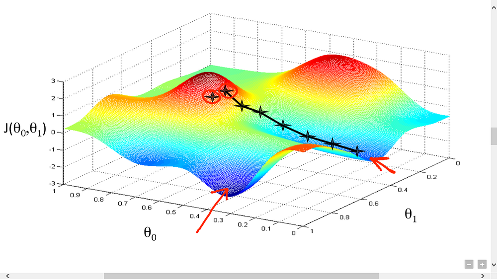
This is an algorithm used in almost every ML model. The Gradient Descent serves to find the minimum of the cost function — which is basically its lowest point or deepest valley. In case you didn’t know, the cost function is a function used to find the errors in the predictions of a Machine Learning model.
Through calculus, you know that the slope of a function is the derivative of the function with respect to a value. With the slope with respect to one weight, you know the direction you need to go to reach the lowest point in the valley. When you iterate data, you need to calculate the slope with respect to each weight. With the averages of the weights, you know where you need to adjust each weight to obtain a minimal standard deviation.
To find out how much you actually need to adjust that weight, you use a Learning Rate, which is called a hyper-parameter. This is basically all trial and error, improved by feeding the neural network more datasets. The cost function should also decrease with every iteration if the Gradient Descent algorithm is working properly. When it can no longer decrease, it is said to have converged.
There are also several different types of gradient descents — which differ in how they handle the datasets — which include:
-
Batch Gradient Descent:This method calculates the margin of error, but only updates the model once the entire dataset has been evaluated. It is computationally efficient, but requires memory, and does not always achieve the most accurate results.
-
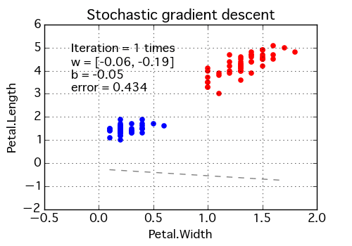
Stochastic Gradient Descent:Instead of updating the model once the dataset has been evaluated, it does so after every training example. The frequent updates allow you to see the detailed improvement until convergence — error rate can vary.
-
Mini-Batch Gradient Descent:This is the method that is used most often in deep learning and training neural networks, and it is a combination of the BGD and the SGD. The dataset is divided into small batches of about 50 to 256, then evaluates each of the batches separately.
 Here is another visual and interactive guide to the basics of neural networks. It’s a great resource to play with the buttons and dials to understand the influence of the weight and bias on the output and error values.
Backpropagating Sums
As mentioned earlier, the sum of the weights can be represented with z = a + b + c + d + … where z is the output and a, b, c, and d… are weighted inputs.
We want to know how much the error will change when we adjust a weight in the network; this can be found through the slope. The error margin and weighted connection between two neurons a, and b can be represented through the following expression:
∂ error/∂ a = (∂ z/∂ a)*(∂ error/∂ z)
For z = a + b + c + d + …, its derivative is 1, which means when one of the input elements is increased by 1, then the output z is also increased by 1.
Backpropagating Sigmoid Functions
Sigmoid is just a fancy word for an S-shaped curve. It’s one of the types of activation function in artificial neurons. If these are present in the neuron, it becomes a sigmoid neuron and not a perceptron. This curve, in terms of machine learning, shows the effect that each of the weights have on the nodes’ output, which will look something like this:
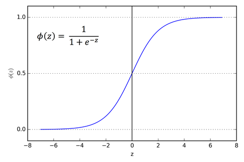
The x-axis represents the value of the input, and the y-axis represents the values of the output of that particular weighted node.
At x = 0, the output of the function is y = 0.5. The sigmoid function always give y-values, or weighted outputs of the nodes, in between 0 and -1. Keep in mind that the weighted outputs refer to outputs within a hidden layer, and not the final output of the neural network itself.
You can tell if a sigmoid neuron is present if there is an S-shape in the artificial neuron diagram. To backpropagate the sigmoid function, we need to find the derivative of its equation. If a is the input neuron and b is the output neuron, the equation is:
b = 1/(1 + e^-x) = σ(a)
This particular function has a property where you can multiply it by 1 minus itself to get its derivative, which looks like this:
σ(a) * (1 — σ(a))
You could also solve the derivative analytically and calculate it if you really wanted to. But because math is amazing and this works too, so hey, why not?
Backpropagating Rectified Linear Units (ReLU)
The effect of the weights can also be represented through a rectified linear function. What that means is all negative weights are just considered as having a value of 0.
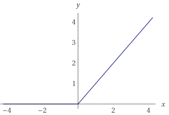
While perceptrons have discrete values of either 0 or 1 and sigmoid neurons have continuous values ranging from 0 to 1, rectified linear units have return only positive values, and are thus defined by the positive parts of its argument. Its values range from 0 to infinity. Similarly to the sigmoid function, the graph of the rectified linear unit shows the x-axis as the value of the input, and the y-axis as the values of the output of that particular weighted node.
If a is the weighted input and b is the weighted output: b = a when a > 0, otherwise b = 0. Then the derivative of the equation is equal to 1 when a > 0, otherwise the derivative is equal to 0.
The Essence of Machine Learning
Now that you’ve learnt some of the main principles of Backpropagation in Machine Learning you understand how it isn’t about having technology come to life so they can abolish the human race. Rather, it’s about teaching them to think, properly recognize trends, and forecast behaviours within the domain of predictive analytics. Reduction in the error rate of the Machine Learning predictions increases its accuracy, allowing it to surpass any human capability. This has great real-world implications because of the wide variety of its applications, and has immense opportunity to grow far beyond anything it can do now.
Bio: Nathalie Jeans is a high school student who is passionate about technology, and currently working on a Handwriting Recognition AI using Neural Networks.
Original. Reposted with permission.
Resources:
Related: