Welcome to part III of debunking the optimism corrected bootstrap in high dimensions (quite high number of features) in the Christmas holidays. Previously we saw with a reproducible code implementation that this method is very bias when we have many features (50-100 or more). I suggest avoiding this method until at some point it has been reassessed thoroughly to find how bad this situation is with different numbers of dimensions. Yes, I know for some statisticians this is your favorite method and they tell people how their method is lacking in statistical power, but clearly this has much worse issues, at least on some data. People are currently using this method in genomic medicine, where we have high numbers of features low samples. Just re-run the code yourself and make up your own mind if in doubt. I have now 3 implementations (excluding Caret) confirming the bias. One written by me, two independent statisticians. Let’s run some more experiments.
This time I have used a different persons implementation using the ‘glm’ function, i.e. logistic regression to show the same misleading trend occurs, i.e. positive results on purely random data. The code has been directly taken from http://cainarchaeology.weebly.com/r-function-for-optimism-adjusted-auc.html, here. The second implementation is from another unnamed statistician, there was a bug in their code so I had to correct it, there may be further errors in it so feel free to check.
If you disagree with these findings, please show your own implementation of the method in R (not using Caret) following the same experiment of increasing number of features that are purely noise very high with binary labels. Also, check the last two posts and re-run the code your self, before making your mind up and providing counter arguments. I am practically certain there is a serious problem with this method. Yet again, with situations like this, don’t rely on Mr X’s publication from 10 years ago, use null simulated data sets with different dimensions to investigate the behavior of the method in question your self.
There are no real predictors in this data, all of them are random data from a normal distribution. The bias is less bad using glm than with glmnet. This method is being used (with high numbers of features) as we speak by Mr Fudge and his friends so they can get into better journals. The system is corrupt.
You should be able to copy and paste this code directly into R to repeat the results. I can’t vouch for this code because I did not write it, but both implementations show the same result as in the last blog post with my code.
Implementation 1. A glm experiment.
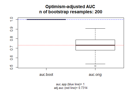
Let’s have a look at the results, which agree nicely with our previous findings using a from scratch implementation of the method. So the red line is supposedly our corrected AUC, but the AUC should be 0.5 when running on random data. See previous part 1 post and part 2 post for demonstration of cross validation results on random data which give the correct result.


Implementation 2: Another glmnet experiment
Here are the results of the above code on random data only (pure madness).
There is some disagreement how to implement this method in Caret as Davis Vaughan disagrees with doing it the way shown here. So, until Max Kuhn gets back to me, relying on the last two posts, I think all the evidence points to a massive positive bias in peoples results using this method with high numbers of features.
If in doubt compare your results with LOOCV and k fold cross validation, this is how I discovered this method is dodgy by seeing MASSIVE differences on null data-sets where no real predictive ability should be found. These two methods are more widely used and reliable.
Sorry @ Frank Harrell, I don’t have time atm to do the extra bits you suggest.Game on @ Davis Vaughan. Do your own implementation with the same data as I have used with glmnet and glm.
The steps of this method, briefly, are as follows:
- Fit a model M to entire data S and estimate predictive ability C.
Iterate from b=1…B:
-
Take a resample from the original data, S*
-
Fit the bootstrap model M* to S* and get predictive ability, C_boot
-
Use the bootstrap model M* to get predictive ability on S, C_orig
Related