By Cecelia Shao, Comet.ml
In this tutorial, we will illustrate how to build an image recognition model using a convolutional neural network (CNN) implemented in MXNet Gluon, and integrate Comet.ml for experiment tracking and monitoring. We will be using the MXNet ResNet model architecture and training that model on the CIFAR 10 dataset for our image classification use case.
MXNet is a deep learning framework that offers optimizations for multi-GPU training and accelerates model development with predefined layers and automatic differentiation. Since MXNet was constructed with large-scale neural networks in mind, the framework is designed for both efficiency and flexibility.
Whether MXNet is an entirely new framework for you or you have used the MXNet backend while training your Keras models, this tutorial illustrates how to build an image recognition model with an MXNet resnet_v1 model.
About the model architecture
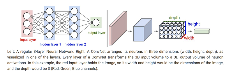
CNNs are a specific category of neural networks that work well with data that has a spatial relationship, making them popular for text data and time-series data, in addition to image data. CNNs are basically just several layers of convolutions with nonlinear activation functions like ReLU or tanh applied to the results. Unlike other neural networks that use fully connected layers, CNNs use convolutions over the input layer to compute the output. This results in local connections, where each region of the input is connected to a neuron in the output. This architecture greatly reduces the number of parameters in the network and allows for a more efficient forward function implementation.
We are using the ResNet CNN architecture for our tutorial because it allows us to have a deeper architecture without sacrificing performance due to the vanishing gradient problem. It solves this problem by introducing “shortcut connections” to fit the input from the previous layer to the next layer without any modification to the input. ResNet’s claim to fame was winning 1st place in the ILSVRC 2015 classification competition and appeared in the He et. al 2015 paper. Although ResNet was originally used for the ImageNet problem, for this tutorial, we’re adapting it to CIFAR-10.
About the data
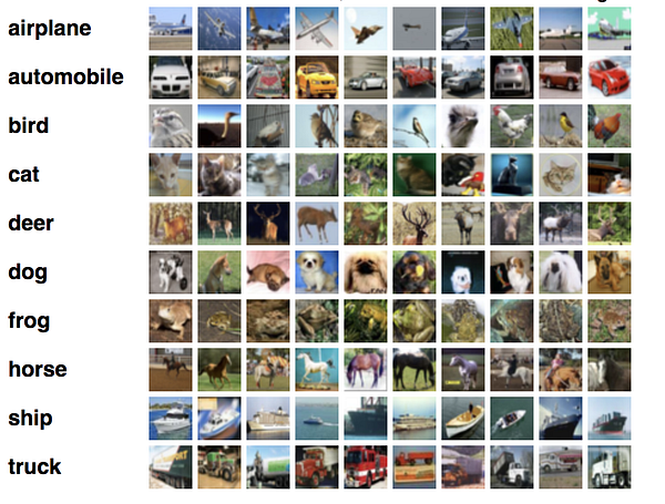
The CIFAR 10 dataset is a labeled subset of the 80 million tiny images dataset It contains 10 mutually exclusive classes (including dogs, cats, planes, automobiles, planes, etc…) with 6,000 images per class. The dataset is divided into five training batches and one test batch so that the test batch contains 1,000 randomly-selected images from each class.
During our training experiments, we’ll explore and adjust different hyperparameters. Since each training session for a particular hyperparameter configuration creates a new model, it becomes harder to manage these as we make progress. This tutorial will also show the use of Comet.ml which allows us to monitor and track our experimentation work.
**Tutorial Step Overview**
We will provide a step-by-step overview next, but if you would like to download the entire script, you can do so here.
First we’ll need to make sure we have the right environment to run the training code:
Hardware:We recommend using a machine with at least 1 GPU to expedite the training process. If you don’t have a GPU available you can also train it on a CPU but training will be very slow. Simply set the num_gpu argument to 0 when you run the script and it will default to using CPUs. See an example command below:
Software: Make sure your environment has the proper library versions installed: Install MXNet by following the instructions available here Install GluonCV by running
Install Comet-ml by running
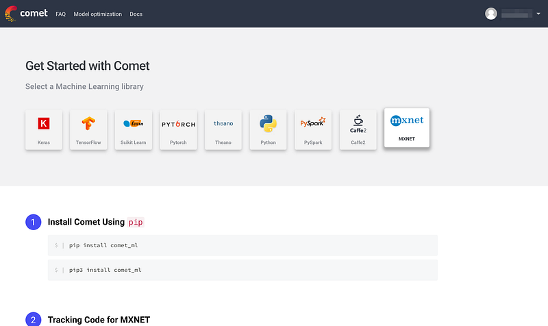
Next, we’ll set up a Comet account and project so we can track the results of our different model iterations. Go to www.comet.ml and sign up with either your email address or Github account.Once you select a plan, you will see a project Quickstart Guide that contains your Comet API key for your project
Now that we have our environment ready we can finally start building our model! Note that the steps we just went through will only need to happen once.
**Code overview:**
We’ll begin by importing with the different libraries we need. Make sure to import comet_ml at the top of your file. We also define the Comet experiment at the top with the API Key you obtained in Step 2 above and your project and workshop name.
As noted in Step 1, we recommend using at least 1 GPU to train this model. Set the - -num_gpus = 1 and define the context to establish what GPU to use.
Next, we’ll set up our data augmentation. Data augmentation both increases the amount of training data and is a great technique for reducing overfitting on models. For more details on data augmentation in gluon, you can refer to this tutorial. Here, we’ll be resizing, cropping, flipping, adjusting the lighting, and using other augmentation techniques on our CIFAR-10 dataset. These transformation operations will be randomized for training, but not during our prediction step.
For our learning rate, we define a decay factor, lr_decay, and the epochs where the learning rate decays. We pay special attention to the learning rate since it controls how much we are adjusting the weights of our network with respect to the loss gradient and ultimately can have an impact on how quickly our model converges to a local minima. A good learning rate can help cut down on the time it takes to train the model.
For our model, we’re using the cifar_restnet20_v1 model architecture available from the MXNet gluoncv model zoo. We’ll use the Nesterov accelerated gradient descent algorithm for our optimizer. Nesterov accelerated gradient uses a “gamble, correct” approach to updating gradients where it uses momentum and the previously calculated gradient to make an informed update to the next gradient that can be corrected later. You can read more about the Nesterov accelerated gradient here.
We can also set the cadence at which our model saves with save_period.
Now we’ll actually split out the data and labels for the validation dataset and define our model evaluation metrics around accuracy.
Finally, we’ll implement the function for training our model. Our train function includes the data loaders for our train and validation data. Since we’re dealing with a single label, multi-class classification problem, we will use the softmax cross entropy loss function.
You’ll notice we added in a line around tracking our model’s training error and validation error.