By Pedro Marcelino, Scientist, Engineer & Entrepreneur
Deep learning is fast becoming a key instrument in artificial intelligence applications (LeCun et al. 2015). For example, in areas such as computer vision, natural language processing, and speech recognition, deep learning has been producing remarkable results. Therefore, there is a growing interest in deep learning.
One of the problems where deep learning excels is image classification(Rawat & Wang 2017). The goal in image classification is to classify a specific picture according to a set of possible categories. A classic example of image classification is the identification of cats and dogs in a set of pictures (e.g. Dogs vs. Cats Kaggle Competition).
From a deep learning perspective, the image classification problem can be solved through transfer learning. Actually, several state-of-the-art results in image classification are based on transfer learning solutions (Krizhevsky et al. 2012, Simonyan & Zisserman 2014, He et al. 2016). A comprehensive review on transfer learning is provided by Pan & Yang (2010).
This article shows how to implement a transfer learning solution for image classification problems. The implementation proposed in this article is based on Keras (Chollet 2015), which uses the programming language Python. Following this implementation, you will be able to solve any image classification problem quickly and easily.
The article has been organised in the following way:
Transfer learning Convolutional neural networks Repurposing a pre-trained model Transfer learning process Classifiers on top of deep convolutional neural networks Example Summary References
1. Transfer learning
Transfer learning is a popular method in computer vision because it allows us to build accurate models in a timesaving way (Rawat & Wang 2017). With transfer learning, instead of starting the learning process from scratch, you start from patterns that have been learned when solving a different problem. This way you leverage previous learnings and avoid starting from scratch. Take it as the deep learning version of Chartres’ expression ‘standing on the shoulder of giants’.
In computer vision, transfer learning is usually expressed through the use of pre-trained models. A pre-trained model is a model that was trained on a large benchmark dataset to solve a problem similar to the one that we want to solve. Accordingly, due to the computational cost of training such models, it is common practice to import and use models from published literature (e.g. VGG, Inception, MobileNet). A comprehensive review of pre-trained models’ performance on computer vision problems using data from the ImageNet (Deng et al. 2009) challenge is presented by Canziani et al. (2016).
2. Convolutional neural networks
Several pre-trained models used in transfer learning are based on large convolutional neural networks (CNN)(Voulodimos et al. 2018). In general, CNN was shown to excel in a wide range of computer vision tasks (Bengio 2009). Its high performance and its easiness in training are two of the main factors driving the popularity of CNN over the last years.
A typical CNN has two parts:
Convolutional base, which is composed by a stack of convolutional and pooling layers. The main goal of the convolutional base is to generate features from the image. For an intuitive explanation of convolutional and pooling layers, please refer to Chollet (2017). Classifier, which is usually composed by fully connected layers. The main goal of the classifier is to classify the image based on the detected features. A fully connected layer is a layer whose neurons have full connections to all activation in the previous layer.
Figure 1 shows the architecture of a model based on CNN. Note that this is a simplified version, which fits the purposes of this text. In fact, the architecture of this type of model is more complex than what we suggest here.
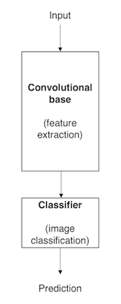 Figure 1. Architecture of a model based on CNN.
One important aspect of these deep learning models is that they can automatically learn hierarchical feature representations. This means that features computed by the first layer are general and can be reused in different problem domains, while features computed by the last layer are specific and depend on the chosen dataset and task. According to Yosinski et al. (2014), ‘if first-layer features are general and last-layer features are specific, then there must be a transition from general to specific somewhere in the network’. As a result, the convolutional base of our CNN — especially its lower layers (those who are closer to the inputs) — refer to general features, whereas the classifier part, and some of the higher layers of the convolutional base, refer to specialised features.
3. Repurposing a pre-trained model
When you’re repurposing a pre-trained model for your own needs, you start by removing the original classifier, then you add a new classifier that fits your purposes, and finally you have to fine-tune your model according to one of three strategies:
Train the entire model. In this case, you use the architecture of the pre-trained model and train it according to your dataset. You’re learning the model from scratch, so you’ll need a large dataset (and a lot of computational power). Train some layers and leave the others frozen.As you remember, lower layers refer to general features (problem independent), while higher layers refer to specific features (problem dependent). Here, we play with that dichotomy by choosing how much we want to adjust the weights of the network (a frozen layer does not change during training). Usually, if you’ve a small dataset and a large number of parameters, you’ll leave more layers frozen to avoid overfitting. By contrast, if the dataset is large and the number of parameters is small, you can improve your model by training more layers to the new task since overfitting is not an issue. Freeze the convolutional base.This case corresponds to an extreme situation of the train/freeze trade-off. The main idea is to keep the convolutional base in its original form and then use its outputs to feed the classifier. You’re using the pre-trained model as a fixed feature extraction mechanism, which can be useful if you’re short on computational power, your dataset is small, and/or pre-trained model solves a problem very similar to the one you want to solve.
Figure 2 presents these three strategies in a schematic way.
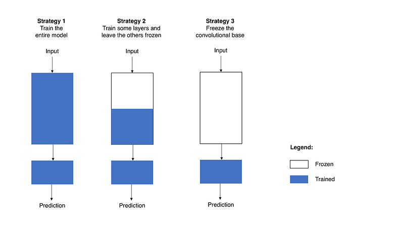 Figure 2. Fine-tuning strategies.
Unlike Strategy 3, whose application is straightforward, Strategy 1andStrategy 2 require you to be careful with the learning rate used in the convolutional part. The learning rate is a hyper-parameter that controls how much you adjust the weights of your network. When you’re using a pre-trained model based on CNN, it’s smart to use a small learning rate because high learning rates increase the risk of losing previous knowledge. Assuming that the pre-trained model has been well trained, which is a fair assumption, keeping a small learning rate will ensure that you don’t distort the CNN weights too soon and too much.
4. Transfer learning process
From a practical perspective, the entire transfer learning process can be summarised as follows:
Select a pre-trained model. From the wide range of pre-trained models that are available, you pick one that looks suitable for your problem. For example, if you’re using Keras, you immediately have access to a set of models, such as VGG (Simonyan & Zisserman 2014), InceptionV3 (Szegedy et al. 2015), and ResNet5 (He et al. 2015). Here you can see all the models available on Keras. Classify your problem according to the Size-Similarity Matrix. In Figure 3 you have ‘The Matrix’ that controls your choices. This matrix classifies your computer vision problem considering the size of your dataset and its similarity to the dataset in which your pre-trained model was trained. As a rule of thumb, consider that your dataset is small if it has less than 1000 images per class. Regarding dataset similarity, let common sense prevail. For example, if your task is to identify cats and dogs, ImageNet would be a similar dataset because it has images of cats and dogs. However, if your task is to identify cancer cells, ImageNet can’t be considered a similar dataset. Fine-tune your model.Here you can use the Size-Similarity Matrix to guide your choice and then refer to the three options we mentioned before about repurposing a pre-trained model. Figure 4 provides a visual summary of the text that follows.
Quadrant 1. Large dataset, but different from the pre-trained model’s dataset. This situation will lead you to Strategy 1. Since you have a large dataset, you’re able to train a model from scratch and do whatever you want. Despite the dataset dissimilarity, in practice, it can still be useful to initialise your model from a pre-trained model, using its architecture and weights. Quadrant 2. Large dataset and similar to the pre-trained model’s dataset. Here you’re in la-la land. Any option works. Probably, the most efficient option is Strategy 2. Since we have a large dataset, overfitting shouldn’t be an issue, so we can learn as much as we want. However, since the datasets are similar, we can save ourselves from a huge training effort by leveraging previous knowledge. Therefore, it should be enough to train the classifier and the top layers of the convolutional base. Quadrant 3. Small dataset and different from the pre-trained model’s dataset. This is the 2–7 off-suit hand of computer vision problems. Everything is against you. If complaining is not an option, the only hope you have is Strategy 2. It will be hard to find a balance between the number of layers to train and freeze. If you go to deep your model can overfit, if you stay in the shallow end of your model you won’t learn anything useful. Probably, you’ll need to go deeper than in Quadrant 2 and you’ll need to consider data augmentation techniques (a nice summary on data augmentation techniques is provided here). Quadrant 4. Small dataset, but similar to the pre-trained model’s dataset. I asked Master Yoda about this one he told me that ‘be the best option, Strategy 3 should’. I don’t know about you, but I don’t underestimate the Force. Accordingly, go for Strategy 3. You just need to remove the last fully-connected layer (output layer), run the pre-trained model as a fixed feature extractor, and then use the resulting features to train a new classifier.
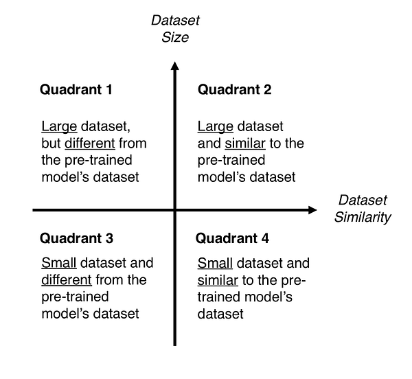
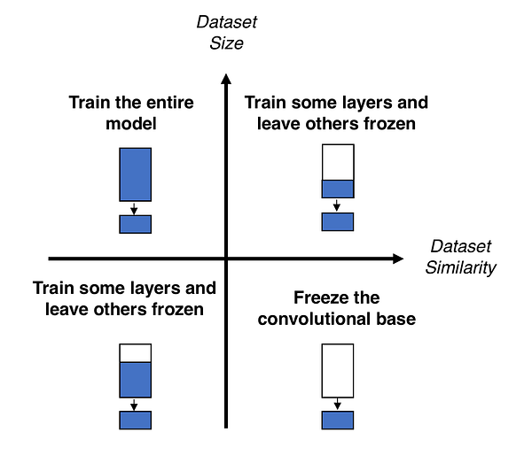 Figures 3 and 4. Size-Similarity matrix (left) and decision map for fine-tuning pre-trained models (right).
5. Classifiers on top of deep convolutional neural networks
As mentioned before, models for image classification that result from a transfer learning approach based on pre-trained convolutional neural networks are usually composed of two parts:
Convolutional base, which performs feature extraction. Classifier, which classifies the input image based on the features extracted by the convolutional base.
Since in this section we focus on the classifier part, we must start by saying that different approaches can be followed to build the classifier. Some of the most popular are:
Fully-connected layers.For image classification problems, the standard approach is to use a stack of fully-connected layers followed by a softmax activated layer (Krizhevsky et al. 2012, Simonyan & Zisserman 2014, Zeiler & Fergus 2014). The softmax layer outputs the probability distribution over each possible class label and then we just need to classify the image according to the most probable class. Global average pooling.A different approach, based on global average pooling, is proposed by Lin et al. (2013). In this approach, instead of adding fully connected layers on top of the convolutional base, we add a global average pooling layer and feed its output directly into the softmax activated layer. Lin et al. (2013) provides a detailed discussion on the advantages and disadvantages of this approach. Linear support vector machines. Linear support vector machines (SVM) is another possible approach. According to Tang (2013), we can improve classification accuracy by training a linear SVM classifier on the features extracted by the convolutional base. Further details about the advantages and disadvantages of the SVM approach can be found in the paper.