By Jay Budzik, Chief Technology Officer, ZestFinance
Advanced machine learning (ML) is a subset of AI that uses more data and sophisticated math to make better predictions and decisions. It’s what powers self-driving cars, Netflix recommendations, and a lot of bank fraud detection. Banks and lenders could make a lot more money using ML on top of legacy credit scoring techniques to find better borrowers and reject more bad ones. But adoption of ML has been held back by the technology’s “black-box” nature. ML models are exceedingly complex. You can’t run a credit model safely or accurately if you can’t explain its decisions.
What we really want from AI explainability are three things: consistency, accuracy, and performance. A handful of techniques are being promoted in the market claiming to solve this “black-box” problem. Caveat emptor. The techniques are often inconsistent, inaccurate, computationally expensive, and/or fail to spot unacceptable outcomes such as race- and gender-based discrimination. Some of these techniques have been in use for a long time, and are quite effective on old modeling approaches such as logistic regression. But they don’t work well with ML.
At ZestFinance, we’ve built new kinds of explainability math into our ZAML software tools that quickly render the inner workings of ML models transparent from creation through deployment. You can use these tools to monitor model health in run-time. You can trust the results are fair and accurate. And we’ve automated the reporting so all you have to do is push a button and produce all the documentation required to comply with regulations.
In this paper, we compare a few popular explainability techniques (including our ZAML technology), describe their relative strengths and weaknesses, and show how each technique stacks up on a simple modeling problem. The test we ran showed that ZAML is more accurate, consistent, and faster than any of these other approaches.
Four Kinds of Explainability Techniques, Explained
Three common ML explainability techniques being championed today are known as LOCO, permutation impact, and LIME. LOCO, which stands for “leave one column out,” substitutes “missing” for a variable and recomputes the model’s prediction. The idea is that if the score changes a lot, the variable that was left out must be really important. Permutation impact (PI), also called permutation importance, substitutes a variable with a randomly selected value and recomputes the model’s prediction. As with LOCO, the idea is that if the score changes a lot, the variable that was scrambled must be really important. LIME, which stands for local interpretable model-agnostic explanations, fits a new linear model in a local neighborhood around a given applicant’s real data values and the real model’s score for those synthetic values. It then uses this new, linear approximation of the actual model to explain how the more complex model behaves. Essentially, you’re taking a very complex model and pretending it’s simple so you can explain it.
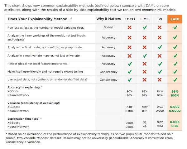
ZestFinance’s ZAML software uses a proprietary explanation method derived from game theory and multivariate calculus that works on the actual underlying model. ZAML explainability determines the relative importance of each variable to the final score by looking at how it interacts with other variables. The checklist below compares these four explainability techniques on seven important capabilities. We also added scores for each of the techniques from a test we ran on their accuracy, consistency and speed at explaining two common ML models. Accuracy is measured by average rank correlation, or how far off the explanations are from the ground truth baselines. Consistency is measured by variance, or how much the difference in explanations varies across all applicants. Speed was the time it took to generate explanations for all the rows in the dataset.
Let’s Unpack This Checklist
Explanations of ML models have to meet a variety of requirements to be trustworthy for high stakes business applications such as credit risk modeling, chief among them accuracy, consistency, and performance, i.e., prediction speed. The chart above summarizes how the four techniques you may be hearing about stack up on an extremely simple model. For real-world explainability problems, such as those endemic to credit risk modeling, the performance differences can be even more pronounced. We used a simple model to demonstrate these differences to make a point that even a model with just two variables can’t be explained by LOCO, PI, or LIME as accurately as ZAML explainability can. If an explainability technique has a hard time explaining the simplest of “toy” models, it may be unwise to trust it on a real-world application where large dollar amounts are at stake.
LOCO, LIME, and PI all have shortcomings with respect to accuracy, consistency, or speed. LOCO and PI work by analyzing one feature one at a time. This means as the number of model variables goes up, the algorithms become slower and more expensive to run. LOCO, LIME, and PI look only at the inputs and outputs of the model, which means they have access to much less information than explainers such as ZAML’s that look at the internal structure of the model. Probing the model externally (i.e. the inputs and outputs) is an imperfect process leading to potential mistakes and inaccuracies. So is analyzing refitted and/or proxy models, as LOCO and LIME require, instead of analyzing your final model. We believe that analyzing the real model is really important - if you don’t you’re opening yourself up to lots of risk.
When attempting to explain advanced ML models, it’s important that your explanations capture the effect of a feature holistically, or in relation to other features. Univariate analysis, as is typically employed with LOCO and PI, will not properly capture these feature interactions and correlation effects. Again, accuracy suffers. Explainers should also calculate feature explanations from a global, and not just local perspective. Let’s say you built a model to understand why Kobe Bryant was a great basketball player. Explaining it using only local feature importance will suggest that his height was not that big of a deal because, from the model’s perspective, all the NBA players clustered around Kobe are also very tall. But you can’t deny that Kobe’s 6’6” height has nothing to do with why he’s so good at basketball. Again, inaccuracies crop up.
Most modeling techniques also have tuning knobs known as hyperparameters that can be automatically dialed in to make a model more accurate. There is no practical equivalent to this “automated tuning” operation for explainers. This makes it really difficult to be confident in the results you get from an explainer like LIME, because there’s no way to tell whether you correctly set a hyperparameter such as the data-area size. Set it too small and the data will be super sparse in the high-dimensional space of all the features in the model. Set it too wide and you will violate the local linear assumption of LIME.
A consistent explainer uses real data. LIME and PI probe the model with non-real data. Let’s say you built a model with income, debt, and debt to income ratio. PI will shuffle each column one at a time independently. This means when PI analyzes debt to income ratio by shuffling, it will no longer be the debt feature divided by the income feature. Since all of the data in the training data maintained this relationship, it should be considered undefined behavior to query a model this way.
Even slight inaccuracies in explanations can lead to devastating outcomes, like releasing models that discriminate based on age, gender, race, or ethnicity, or releasing models that are unstable and produce high default rates that can cause lending businesses to hemorrhage money. A model explainability technique should provide the same answer given the same inputs and model. Inaccurate or inconsistent model explainability techniques might appear to provide some assurance of risk management, but if the results aren’t accurate, they provide little value or assurance to business stakeholders and regulators.
Speed and efficiency are also important. Model explainability should be used often during the model build process and as the model is applied in order to generate explanations for each model-based decision. Slow and inefficient techniques limit the usefulness of explainability: If you have to wait overnight for results, you’re going to run the analysis less often, and get less frequent insights about how your model is working. That means less time working on better models.
Putting Explainability Techniques To The Test
We took our comparison of these four explainability techniques one step further and ran an experiment evaluating how these approaches performed in relation to ground truth on a simple modeling problem. For this test, we used as ground truth a reference value computed using math derived from competitive game theory. The reference value measures the average marginal benefit introduced by a given model’s input variables. It does this by exhaustively enumerating all possible combinations of variables. Computing the reference value requires creating an exponential number of model variations, each with a different combination of variables included. By understanding the comparative performance of the models, we can quantify the value of each variable used in the model.
For our experiment, we evaluated the performance of the four techniques at explaining two ML models and the “moons” dataset. This is a simple, two variable data set with 100,000 rows, and is often used in undergraduate machine learning courses to demonstrate the limitations of linear models.
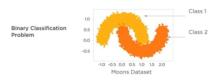
The moons classification task is to build a model that separates the light orange data points from the dark orange data points using only the X and Y coordinates. A linear model simply can’t do this very well. To see this, just draw any straight line through the above diagram and notice that on either side of the line you have both yellow and green data points. There is no straight line that can separate the orange sections. The moons dataset provides a simple example showing that machine learning methods are sensitive to variable interactions and capture the real shape of the data better than old methods like logistic regression that can only create linear models.
We built two machine learning classification models trained on this data set. One using XGBoost, a popular tree ensemble induction algorithm, and Tensorflow, a popular neural network package. At the time of writing, both were considered best in class machine learning modeling techniques. We then applied the various explainability approaches to the resulting tree and neural network models. The results are provided below.
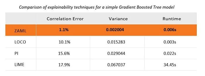
For gradient boosted trees, LIME, PI, and LOCO all produce high error rates and much higher variance even on a very simple modeling problem, when compared with ZAML. Also important to note is that LIME is much slower to compute. While PI and LOCO appear to be more reasonable in this test on a two-variable model, these methods get much slower very quickly as the number of rows and columns increase. For larger datasets such as those we see every day in our credit risk modeling work, they become impractical. We’ve waited hours, even days, for explanations from LOCO, PI, and LIME. In our experience, the ZAML approach doesn’t take more than a few seconds to compute on a single laptop or modest computer, even for models with thousands of variables.
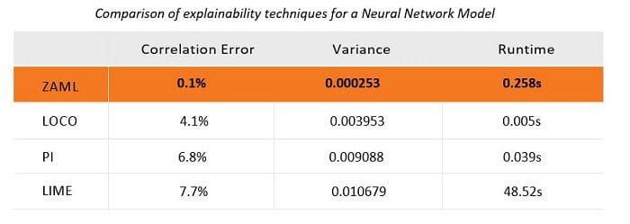
For neural networks, LIME, PI and LOCO also generate much higher error rates and higher variance. Consistent with its performance on gradient boosted trees, LIME is very slow. For those interested, the scatter plots showing the comparison of each method with the reference values are included in the appendix below.
Conclusion
Not all explainability techniques are created equal. Even on a simple modeling problem like the two-dimensional “moons” dataset, with only 100,000 rows, we have shown that ZAML explainability is more accurate, consistent, and often faster than the other approaches. When applying machine learning on high-stakes business problems like credit risk modeling, it’s critical to get the core explainability method right so that you know what your model is doing and can manage the risk associated with its application. If the core explainability math you use generates the wrong answer, you might get your business into serious trouble.
Bio: Jay Budzik is a product and technology leader with track record of driving exceptional revenue growth by applying AI and ML to create new products and services.
Original. Reposted with permission.
Resources:
Related: