When I started my Data Science journey, I casually Googled ‘Application of Machine Learning Algorithms’. For the next 10 minutes, I had my jaw hanging. Quite literally. Part of the reason was that they were all around me. That music video from YouTube recommendations that you ended up playing hundred times on loop? That’s Machine Learning for you. Ever wondered how Google keyboard completes your sentence better than your bestie ever could? Machine Learning again!
So how does this magic happen? What do you need to perform this witchcraft? Before you move further, let me tell you who would benefit from this article.
-
Someone who has just begun her/his Data Science journey and is looking for theory and application on the same platter.
-
Someone who has a basic idea of probability and linear algebra.
-
Someone who wants a brief mathematical understanding of ML and not just a small talk like the one you did with your neighbour this morning.
-
Someone who aims at preparing for a Data Science job interview.
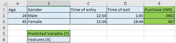
‘Machine Learning’ literally means that a machine (in this case an algorithm running on a computer) learns from the data it is fed. For example, you have customer data for a supermarket. The data consists of customers age, gender, time of entry and exit and the total purchase. You train a Machine Learning algorithm to learn the purchase pattern of customers and predict the purchase amount for a new customer by asking for his age, gender, time of entry and exit.
Now, Let’s dig deep and explore the workings of it.
Machine Learning (ML) Algorithms
Before we talk about the various classes, let us define some terms:
Seen data or Train Data –
This is all the information we have. For example, data of 1000 customers with their age, gender, time of entry and exit and their purchases.
Predicted Variable (or Y) –
The ML algorithm is trained to predict this variable. In our example, the ‘Purchase amount’. The predicted variable is usually called the dependent variable.
Features (or X) –
Everything in the data except for Y. Basically, the input that is fed to the model. Features are usually called the independent variable.
Model Parameters –
Parameters define our ML model. This will be understood later as we discuss each model. For now, remember that our main goal is to evaluate these parameters.
Unseen data or Test Data–
This is the data for which we have the X but not Y. The why has to be predicted using the ML model trained on the seen data.
Now that we have defined our terms, let’s move to the classes of Machine Learning or ML algorithms.
Supervised Learning Algorithms:
These algorithms require you to feed the data along with the predicted variable. The parameters of the model are then learned from this data in such a way that error in prediction is minimized. This will be more clear when individual algorithms are discussed.
Unsupervised Learning Algorithms:
These algorithms do not require data with predicted variables. Then what do we predict? Nothing. We just cluster these data points.
If you have any doubts about the things discussed above, keep on reading. It will get clearer as you see examples.
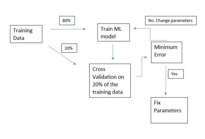
Cross-validation :
A general strategy used for setting parameters for any ML algorithm in general. You take out a small part of your training (seen) data, say 20%. You train an ML model on the 80% and then check it’s performance on that 20% of data (remember you have the Y values for this 20 %). You tweak the parameters until you get minimum error. Take a look at the flowchart below.
Supervised Learning Algorithms
In Supervised Machine Learning, there are two types of predictions – Regression or Classification. Classification means predicting classes of a data point. For example – Gender, Type of flower, Whether a person will pay his credit card bill or not. The predicted variable has 2 or more possible discrete values. Regression means predicting a numeric value of a data point. For example – Purchase amount, Age of a person, Price of a house, Amount of predicted rainfall, etc. The predicted class is a continuous variable. A few algorithms perform one of either task. Others can be used for both the tasks. I will mention the same for each algorithm we discuss. Let’s start with the most simple one and slowly move to more complex algorithms.
KNN: K-Nearest Neighbours
“You are the average of 5 people you surround yourself with”**-John Rim
Congratulations! You just learned your first ML algorithm.
Don’t believe me? Let’s prove it!
Consider the case of classification. Let’s set K, which is the number of closest neighbours to be considered equal to 3. We have 6 seen data points whose features are height and weight of individuals and predicted variable is whether or not they are obese.
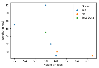
Consider a point from the unseen data (in green). Our algorithm has to predict whether the person represented by the green data point is obese or not. If we consider it’s K(=3) nearest neighbours, we have 2 obese (blue) and one not obese (orange) data points. We take the majority vote of these 3 neighbours which is ‘Yes’. Hence, we predict this individual to be obese. In case of regression, everything remains the same, except that we **take the average **of the Y values of our K neighbours. How to set the value of K? Using cross-validation.
Key facts about KNN:
-
KNN performs poorly in higher dimensional data, i.e. data with too many features.(Curse of dimenstionality)
-
Euclidean distance is used for computing distance between continuous variables. If the data has categorical variables (gender, for example), Hamming distance is used for such variables. There are many popular distance measures used apart from these. You can find a detailed explanation here.
Linear Regression
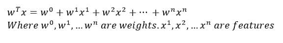
This is yet another simple, but an extremely powerful model. It is only used for regression purposes. It is represented by
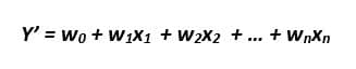
….(1)
Y’ is the value of the predicted variable according to the model. X1, X2,…Xn are input features. Wo, W1..Wn are the parameters (also called weights) of the model. Our aim is to estimate the parameters from the training data to completely define the model.
How do we do that? Let’s start with our objective which is to minimize the error in the prediction of our target variable. How do we define our error? The most common way is to use the MSE or Mean Squared Error – 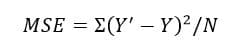
For all N points, we sum the squares of the difference of the predicted value of Y by the model, i.e. Y’ and the actual value of the predicted variable for that point, i.e. Y.
We then replace Y’ with equation (1) and differentiate this MSE with respect to parameters W0,W1..Wn and equate it to 0 to get values of the parameters at which the error is minimum.
An example of how a linear regression might look like is shown below.
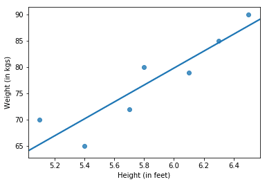
Sometimes it is not necessary that our dependent variable follows linear dependency on our independent variable. For example, Weight in the above graph may vary with the square of Height. This is called polynomial regression (Y varies with some power of X).
Good news is that any polynomial regression can be transformed to linear regression. How?
We transform the independent variable. Take a look at the Height variable in both the tables.

Table 1

table 2
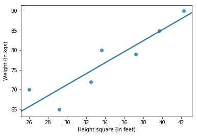
We will forget about Table 1 and treat the polynomial regression problem like a linear regression problem. Only this time, Weight will be linear in Height squared (notice the x-axis in the figure below).
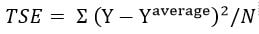
A very important question about every ML model one should ask is – How do you measure the performance of the model? One popular measure is R-squared
R-squared: Intuitively, it measures how well the data and hence the model explains the variation in the dependent variable. How? Consider the following question – If you had just the Y values and no X values in your data, and someone asks you, “Hey! For this X, what would you predict the Y to be?” What would be your best guess? The average of all the Y values you have! In this scenario of limited information, you are better off guessing the average of Y for any X than anything other value of Y.
But, now that you have X and Y values, you want to see how well your linear regression model predicts Y for any unseen X. R-squared quantifies the performance of your linear regression model over this ‘baseline model’
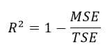
MSE is the mean squared error as discussed before. TSE is the total squared error or the baseline model error.
Naive Bayes
Naive Bayes is a classification algorithm. As the name suggests, it is based on Bayes rule.
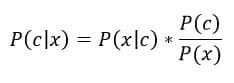
Intuitive Breakdown of Bayes rule: Consider a classification problem where we are asked to predict the class of a data point x. We have two classes and the classes are denoted by letter C.
Now, P(c), also known as the ‘Prior Probability’ is the probability of a data point belonging to class C, when we don’t have any data. For example, if we have 100 roses and 200 sunflowers and someone asks you to classify an unseen flower while providing you with no information, what would you say?
P(rose) = 100/300 = ⅓ P(sunflower) = 200/300 = ⅔
Since P(sunflower) is higher, your best guess would be a sunflower. P(rose) and P(sunflower) are prior probabilities of the two classes.
Now, you have additional information about your 300 flowers. The information is related to thorns on their stem. Look at the table below. |Flower\Thorns|Thorns|No Thorns| |Rose (Total 100)|90|10| |Sunflower (Total 200)|50|150|
Now come back to the unseen flower. You are told that this unseen flower has thorns. Let this information about thorns be X.
| P(rose | X) = 90/100 = 9/10 P(sunflower | X) = 50/150 = ⅓ |
Now according to Bayes rule, the numerator for the two classes are as follows –
Rose = 1/3*9/10 = 3/10 = 0.3
Sunflower = 2/3*1/3 = 2/9 = 0.22
The denominator, P(x), called the evidence is the cumulative probability of seeing the data point itself. In this case it is equal to 0.3 + 0.22 = 0.52. Since it does not depend on the class, it won’t affect our decision-making process. We will ignore it for our purposes.
Since, 0.3>0.22
| P(Rose | X) > P(sunflower | X) |
Therefore, our prediction would be that the unseen flower is a Rose. Notice that our prior probabilities of both the classes favoured Sunflower. But as soon as we factored the data about thorns, our decision changed.
If you understood the above example, you have a fair idea of the Naive Bayes Algorithm.
This simple example where we had only one feature (information about thorns) can be extended to multiple features. Let these features be x1, x2, x3 … xn. Bayes Rule would look like –
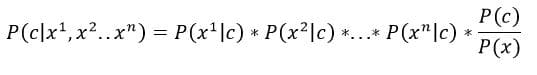
Note that we assume the features to be independent. Meaning,
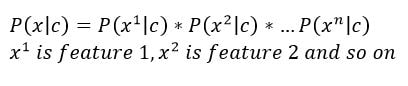
The algorithm is called ‘Naive’ because of the above assumption
Logistic Regression
Logistic regression, unlike its name, is used for classification purposes. The mathematical model used for logistic regression is called the logit function. Consider two classes 0 and 1.
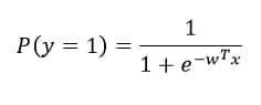
P(y=1) denotes the probability of belonging to class 1 and 1-P(y=1) is thus the probability of the data point belonging to class 0 (notice that the range of the function for all WT*X is between 0 and 1). Like other models, we need to learn the parameters w0, w1, w2, … wn to completely define the model. Like linear regression has MSE to quantify the loss for any error made in the prediction, logistic regression has the following loss function –
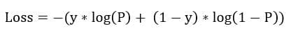
P is the probability of a data point belonging to class 1 as predicted by the model. Y is the actual class of the model.
Think about this – If the actual class of a data point is 1 and the model predicts P to be 1, we have 0 loss. This makes sense. On the other hand, if P was 0 for the same data point, the loss would be -infinity. This is the worst case scenario. This loss function is used in the Gradient Descent Algorithm to reach the parameters at which the loss is minimum.
Okay! So now we have a model that can predict the probability of an unseen data point belonging to class 1. But how do we make a decision for that point? Remember that our final goal is to assign classes, not just probabilities.
At what probability threshold do we say that the point belongs to class 1. Well, the model assigns the class according to the probabilities. If P>0.5, the class if obviously 1. However, we can change this threshold to maximize the metric of our interest ( precision, recall…), we can choose the best threshold using cross-validation.
This was Logistic Regression for you. Of course, do follow the coding tutorial!
Decision Tree
“Suppose there exist two explanations for an occurrence. In this case, the one that requires the least speculation is usually better.” – **Occam’s Razor
The above philosophical principle precisely guides one of the most popular supervised ML algorithm. Decision trees, unlike other algorithms, are non-parametric algorithms. We don’t necessarily need to specify any parameter to completely define the model unlike KNN (where we need to specify K).
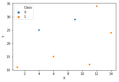
Let’s take an example to understand this algorithm. Consider a classification problem with two classes 1 and 0. The data has 2 features X and Y. The points are scattered on the X-Y plane as

Our job is to make a tree that asks yes or no questions to a feature in order to create classification boundaries. Consider the tree below:
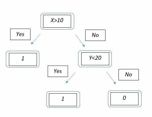
The tree has a ‘Root Node’ which is ‘X>10’. If yes, then the point lands at the leaf node with class 1. Else it goes to the other node where it is asked if its Y value is <20. Depending on the answer, it goes to either of the leaf nodes. Boundaries would look something like –
How to decide which feature should be chosen to bifurcate the data? The concept of ‘Purity ‘ is used here. Basically, we measure how pure (pure in 0s or pure in 1s) our data becomes on both the sides as compared to the node from where it was split. For example, if we have 50 1s and 50 0s at some node. After splitting, we have 40 1s and 10 0s on one side and 10 1s and 40 0s on the other, then we have a good splitting (one node is purer in 1s and the other in 0s). This goodness of splitting is quantified using the concept of Information Gain. Details can be found here.
Conclusion
If you have come so far, awesome job! You now have a fair level of understanding of basic ML algorithms along with their applications in Python. Now that you have a solid foundation, you can easily tackle advanced algorithms like Neural Nets, SVMs, XGBoost and many others.
Happy learning!
Please follow and like us:
![]()