In this tutorial, you will learn how to save and load your Keras deep learning models.
This blog post was inspired by PyImageSearch reader, Mason, who emailed in last week and asked:
Adrian, I’ve been going through your blog and reading your deep learning tutorials. Thanks for them. I have a question though: After training, how do you save your Keras model? And once you have it saved, how do you load it again so you can classify new images? I know this is a basic question but I don’t know how to save and load my Keras models.
Mason asks an excellent question — and it’s actually not as “basic” of a concept as he (and maybe even you) may think.
On the surface, saving your Keras models is as simple as calling the model.save and load_model function. But there’s actually more to consider than just the load and save model functions!
What’s even more important, and sometimes overlooked by new deep learning practitioners, is the preprocessing stage — your preprocessing steps for training and validation must be identical to the training steps when loading your model and classifying new images.
In the remainder of today’s tutorial we’ll be exploring:
-
How to properly save and load your Keras deep learning models.
-
The proper steps to preprocess your images after loading your model.
To learn how to save and load your deep learning models with Keras, just keep reading!
Keras – Save and Load Your Deep Learning Models
In the first part of this tutorial, we’ll briefly review both (1) our example dataset we’ll be training a Keras model on, along with (2) our project directory structure. From there I will show you how to:
-
Train a deep learning model with Keras
-
Serialize and save your Keras model to disk
-
Load your saved Keras model from disk
-
Make predictions on new image data using your saved Keras model
Let’s go ahead and get started!
Our example dataset
The dataset we’ll be utilizing for today’s tutorial is a subset of the malaria detection and classification dataset we covered in last week’s Deep learning and Medical Image Analysis with Keras blog post.
The original dataset consists of 27,588 images belonging to two classes:
-
Parasitized: Implying that the image contains malaria
-
Uninfected: Meaning there is no evidence of malaria in the image
Since the goal of this tutorial is not medical image analysis, but rather how to save and load your Keras models, I have sampled the dataset down to 100 images.
I have reduced the dataset size mainly because:
-
You should be able to run this example on your CPU (if you do not own/have access to a GPU).
-
Our goal here is to teach the basic concept of saving and loading Keras models, not train a state-of-the-art malaria detector.
-
And because of that, it’s better to work with a smaller example dataset
If you would like to read my full blog post on how to build a (near) state-of-the-art malaria classifier with the full dataset, please be sure to refer to this blog post.
Project structure
Be sure to grab today’s “Downloads” consisting of the reduced dataset, ResNet model, and Python scripts.
Once you’ve unzipped the files you’ll be presented with this directory structure:
| 12345678910111213141516171819 | $ tree –filelimit 10 –dirsfirst.├── malaria│ ├── testing│ │ ├── Parasitized [50 entries]│ │ └── Uninfected [50 entries]│ ├── training│ │ ├── Parasitized [175 entries]│ │ └── Uninfected [185 entries]│ └── validation│ ├── Parasitized [18 entries]│ └── Uninfected [22 entries]├── pyimagesearch│ ├── init.py│ └── resnet.py├── save_model.py└── load_model.py 11 directories, 4 files |
2
4
6
8
10
12
14
16
18
.
│ ├── testing
│ │ └── Uninfected [50 entries]
│ │ ├── Parasitized [175 entries]
│ └── validation
│ └── Uninfected [22 entries]
│ ├── init.py
├── save_model.py
Our project consists of two folders in the root directory:
malaria/ : Our reduced Malaria dataset. It is organized into training, validation, and testing sets via the “build dataset” script from last week.
pyimagesearch/ : A package included with the downloads which contains our ResNet model class.
Today, we’ll review two Python scripts as well:
save_model.py : A demo script which will save our Keras model to disk after it has been trained.
load_model.py : Our script that loads the saved model from disk and classifies a small selection of testing images.
By reviewing these files, you’ll quickly see how easy Keras makes saving and loading deep learning model files.
Saving a model with Keras
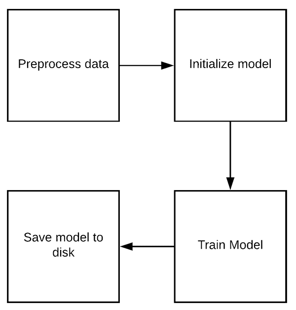
Figure 2: The steps for training and saving a Keras deep learning model to disk.
Before we can load a Keras model from disk we first need to:
-
Train the Keras model
-
Save the Keras model
The save_model.py script we’re about to review will cover both of these concepts.
Go ahead and open up your save_model.py file and let’s get started:
| # set the matplotlib backend so figures can be saved in the backgroundimport matplotlibmatplotlib.use(“Agg”) # import the necessary packagesfrom keras.preprocessing.image import ImageDataGeneratorfrom keras.optimizers import SGDfrom pyimagesearch.resnet import ResNetfrom sklearn.metrics import classification_reportfrom imutils import pathsimport matplotlib.pyplot as pltimport numpy as npimport argparseimport os |
import matplotlib
from keras.preprocessing.image import ImageDataGenerator
from pyimagesearch.resnet import ResNet
from imutils import paths
import numpy as np
import os
We begin on Lines 2-14 by importing required packages.
On Line 3 the “Agg” matplotlib backend is specified as we’ll be saving our plot to disk (in addition to our model).
Our ResNet CNN is imported on Line 8. In order to use this CNN, be sure to grab the “Downloads” for today’s blog post.
Using the argparse import, let’s parse our command line arguments:
| # construct the argument parser and parse the argumentsap = argparse.ArgumentParser()ap.add_argument(“-d”, “–dataset”, type=str, required=True, help=”path dataset of input images”)ap.add_argument(“-m”, “–model”, type=str, required=True, help=”path to trained model”)ap.add_argument(“-p”, “–plot”, type=str, default=”plot.png”, help=”path to output loss/accuracy plot”)args = vars(ap.parse_args()) |
ap = argparse.ArgumentParser()
help=”path dataset of input images”)
help=”path to trained model”)
help=”path to output loss/accuracy plot”)
Our script requires that three arguments be provided with the command string in your terminal:
–dataset : The path to our dataset. We’re using a subset of the Malaria dataset that we built last week.
–model : You need to specify the path to the trained output model (i.e., where the Keras model is going to be saved). This is key for what we are covering today.
–plot : The path to the training plot. By default, the figure will be named plot.png .
No modifications are needed for these lines of code. Again, you will need to type the values for the arguments in the terminal and let argparse do the rest. If you are unfamiliar with the concept of command line arguments, see this post.
Let’s initialize our training variables and paths:
| 262728293031323334353637383940 | # initialize the number of training epochs and batch sizeNUM_EPOCHS = 25BS = 32 # derive the path to the directories containing the training,# validation, and testing splits, respectivelyTRAIN_PATH = os.path.sep.join([args[“dataset”], “training”])VAL_PATH = os.path.sep.join([args[“dataset”], “validation”])TEST_PATH = os.path.sep.join([args[“dataset”], “testing”]) # determine the total number of image paths in training, validation,# and testing directoriestotalTrain = len(list(paths.list_images(TRAIN_PATH)))totalVal = len(list(paths.list_images(VAL_PATH)))totalTest = len(list(paths.list_images(TEST_PATH))) |
27
29
31
33
35
37
39
NUM_EPOCHS = 25
validation, and testing splits, respectively
VAL_PATH = os.path.sep.join([args[“dataset”], “validation”])
and testing directories
totalVal = len(list(paths.list_images(VAL_PATH)))
We’ll be training for 25 epochs with a batch size of 32 .
Last week, we split the NIH Malaria Dataset into three sets, creating a corresponding directory for each:
-
Training
-
Validation
-
Testing
Be sure to review the build_dataset.py script in the tutorial if you’re curious how the data split process works. For today, I’ve taken the resulting dataset that has been split (as well as made is significantly smaller for the purposes of this blog post).
The images paths are built on Lines 32-34, and the number of images in each split is grabbed on Lines 38-40.
Let’s initialize our data augmentation objects:
| 42434445464748495051525354 | # initialize the training training data augmentation objecttrainAug = ImageDataGenerator( rescale=1 / 255.0, rotation_range=20, zoom_range=0.05, width_shift_range=0.05, height_shift_range=0.05, shear_range=0.05, horizontal_flip=True, fill_mode=”nearest”) # initialize the validation (and testing) data augmentation objectvalAug = ImageDataGenerator(rescale=1 / 255.0) |
43
45
47
49
51
53
trainAug = ImageDataGenerator(
rotation_range=20,
width_shift_range=0.05,
shear_range=0.05,
fill_mode=”nearest”)
initialize the validation (and testing) data augmentation object
Data augmentation is the process of generating new images from a dataset with random modifications. It results in a better deep learning model and I almost always recommend it (it is especially important for small datasets).
Data augmentation is briefly covered in my Keras Tutorial blog post. For a full dive into data augmentation be sure to read my deep learning book, Deep Learning for Computer Vision with Python.
Note: The valAug object simply performs scaling — no augmentation is actually performed. We’ll be using this object twice: once for validation rescaling and once for testing rescaling.
Now that the training and validation augmentation objects are created, let’s initialize the generators:
| 5354555657585960616263646566676869707172737475767778 | # initialize the training generatortrainGen = trainAug.flow_from_directory( TRAIN_PATH, class_mode=”categorical”, target_size=(64, 64), color_mode=”rgb”, shuffle=True, batch_size=BS) # initialize the validation generatorvalGen = valAug.flow_from_directory( VAL_PATH, class_mode=”categorical”, target_size=(64, 64), color_mode=”rgb”, shuffle=False, batch_size=BS) # initialize the testing generatortestGen = valAug.flow_from_directory( TEST_PATH, class_mode=”categorical”, target_size=(64, 64), color_mode=”rgb”, shuffle=False, batch_size=BS) |
54
56
58
60
62
64
66
68
70
72
74
76
78
trainGen = trainAug.flow_from_directory(
class_mode=”categorical”,
color_mode=”rgb”,
batch_size=BS)
initialize the validation generator
VAL_PATH,
target_size=(64, 64),
shuffle=False,
testGen = valAug.flow_from_directory(
class_mode=”categorical”,
color_mode=”rgb”,
batch_size=BS)
The three generators above actually produce images on demand during training/validation/testing per our augmentation objects and the parameters given here.
Now we’re going to build, compile, and train our model. We’ll also evaluate our model and print a classification report:
| 8384858687888990919293949596979899100101102103104105106107108109110111 | # initialize our Keras implementation of ResNet model and compile itmodel = ResNet.build(64, 64, 3, 2, (2, 2, 3), (32, 64, 128, 256), reg=0.0005)opt = SGD(lr=1e-1, momentum=0.9, decay=1e-1 / NUM_EPOCHS)model.compile(loss=”binary_crossentropy”, optimizer=opt, metrics=[“accuracy”]) # train our Keras modelH = model.fit_generator( trainGen, steps_per_epoch=totalTrain // BS, validation_data=valGen, validation_steps=totalVal // BS, epochs=NUM_EPOCHS) # reset the testing generator and then use our trained model to# make predictions on the dataprint(“[INFO] evaluating network…“)testGen.reset()predIdxs = model.predict_generator(testGen, steps=(totalTest // BS) + 1) # for each image in the testing set we need to find the index of the# label with corresponding largest predicted probabilitypredIdxs = np.argmax(predIdxs, axis=1) # show a nicely formatted classification reportprint(classification_report(testGen.classes, predIdxs, target_names=testGen.class_indices.keys())) |
84
86
88
90
92
94
96
98
100
102
104
106
108
110
model = ResNet.build(64, 64, 3, 2, (2, 2, 3),
opt = SGD(lr=1e-1, momentum=0.9, decay=1e-1 / NUM_EPOCHS)
metrics=[“accuracy”])
train our Keras model
trainGen,
validation_data=valGen,
epochs=NUM_EPOCHS)
reset the testing generator and then use our trained model to
print(“[INFO] evaluating network…”)
predIdxs = model.predict_generator(testGen,
label with corresponding largest predicted probability
print(classification_report(testGen.classes, predIdxs,
In the code block above, we:
Initialize our implementation of ResNet on Lines 84-88 (from Deep Learning for Computer Vision with Python). Notice how we’ve specified “binary_crossentropy” because our model has two classes. You should change it to “categorical_crossentropy” if you are working with > 2 classes. Train the ResNet model on the augmented Malaria dataset (Lines 91-96).
- Make predictions on test set (Lines 102 and 103) and extract the highest probability class index for each prediction (Line 107).
Display a classification_report in our terminal (Lines 110-111).
Now that our model is trained let’s save our Keras model to disk:
| # save the network to diskprint(“[INFO] serializing network to ‘{}’…“.format(args[“model”]))model.save(args[“model”]) |
print(“[INFO] serializing network to ‘{}’…“.format(args[“model”]))
To save our Keras model to disk, we simply call .save on the model (Line 115).
Simple right?
Yes, it is a simple function call, but the hard work before it made the process possible.
In our next script, we’ll be able to load the model from disk and make predictions.
Let’s plot the training results and save the training plot as well:
| 117118119120121122123124125126127128129 | # plot the training loss and accuracyN = NUM_EPOCHSplt.style.use(“ggplot”)plt.figure()plt.plot(np.arange(0, N), H.history[“loss”], label=”train_loss”)plt.plot(np.arange(0, N), H.history[“val_loss”], label=”val_loss”)plt.plot(np.arange(0, N), H.history[“acc”], label=”train_acc”)plt.plot(np.arange(0, N), H.history[“val_acc”], label=”val_acc”)plt.title(“Training Loss and Accuracy on Dataset”)plt.xlabel(“Epoch #”)plt.ylabel(“Loss/Accuracy”)plt.legend(loc=”lower left”)plt.savefig(args[“plot”]) |
118
120
122
124
126
128
N = NUM_EPOCHS
plt.figure()
plt.plot(np.arange(0, N), H.history[“val_loss”], label=”val_loss”)
plt.plot(np.arange(0, N), H.history[“val_acc”], label=”val_acc”)
plt.xlabel(“Epoch #”)
plt.legend(loc=”lower left”)
At this point our script is complete. Let’s go ahead and train our Keras model!
To train your Keras model on our example dataset, make sure you use the “Downloads” section of the blog post to download the source code and images themselves.
From there, open up a terminal and execute the following command:
| 1234567891011121314151617181920212223242526 | $ python save_model.py –dataset malaria –model saved_model.modelFound 360 images belonging to 2 classes.Found 40 images belonging to 2 classes.Found 100 images belonging to 2 classes.Epoch 1/2511/11 [==============================] - 10s 880ms/step - loss: 0.9204 - acc: 0.5686 - val_loss: 7.0116 - val_acc: 0.5625Epoch 2/2511/11 [==============================] - 7s 624ms/step - loss: 0.8821 - acc: 0.5899 - val_loss: 1.4123 - val_acc: 0.4375Epoch 3/2511/11 [==============================] - 7s 624ms/step - loss: 0.9426 - acc: 0.5878 - val_loss: 0.8156 - val_acc: 0.6562…Epoch 23/2511/11 [==============================] - 7s 664ms/step - loss: 0.3372 - acc: 0.9659 - val_loss: 0.2396 - val_acc: 0.9688Epoch 24/2511/11 [==============================] - 7s 622ms/step - loss: 0.3035 - acc: 0.9514 - val_loss: 0.3389 - val_acc: 0.9375Epoch 25/2511/11 [==============================] - 7s 628ms/step - loss: 0.3023 - acc: 0.9465 - val_loss: 0.3954 - val_acc: 0.9375[INFO] evaluating network… precision recall f1-score support Parasitized 1.00 0.98 0.99 50 Uninfected 0.98 1.00 0.99 50 avg / total 0.99 0.99 0.99 100 [INFO] serializing network to ‘saved_model.model’… |
2
4
6
8
10
12
14
16
18
20
22
24
26
Found 360 images belonging to 2 classes.
Found 100 images belonging to 2 classes.
11/11 [==============================] - 10s 880ms/step - loss: 0.9204 - acc: 0.5686 - val_loss: 7.0116 - val_acc: 0.5625
11/11 [==============================] - 7s 624ms/step - loss: 0.8821 - acc: 0.5899 - val_loss: 1.4123 - val_acc: 0.4375
11/11 [==============================] - 7s 624ms/step - loss: 0.9426 - acc: 0.5878 - val_loss: 0.8156 - val_acc: 0.6562
Epoch 23/25
Epoch 24/25
Epoch 25/25
[INFO] evaluating network…
Uninfected 0.98 1.00 0.99 50
avg / total 0.99 0.99 0.99 100
[INFO] serializing network to ‘saved_model.model’…
Notice the command line arguments. I’ve specified the path to the Malaria dataset directory ( –dataset malaria ) and the path to our destination model ( –model saved_model.model ). These command line arguments are key to the operation of this script. You can name your model whatever you’d like without changing a line of code!
Here you can see that our model is obtaining ~99% accuracy on the test set.
Each epoch is taking ~7 seconds on my CPU. On my GPU each epoch takes ~1 second. Keep in mind that training is faster than last week because we’re pushing less data through the network for each epoch due to the fact that I reduced today’s dataset.
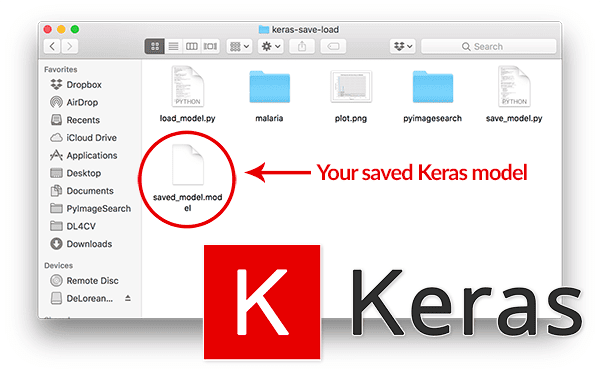
After training you can list the contents of your directory and see the saved Keras model:
| $ ls -ltotal 5216-rw-r–r–@ 1 adrian staff 2415 Nov 28 10:09 load_model.pydrwxr-xr-x@ 5 adrian staff 160 Nov 28 08:12 malaria-rw-r–r–@ 1 adrian staff 38345 Nov 28 10:13 plot.pngdrwxr-xr-x@ 6 adrian staff 192 Nov 28 08:12 pyimagesearch-rw-r–r–@ 1 adrian staff 4114 Nov 28 10:09 save_model.py-rw-r–r–@ 1 adrian staff 2614136 Nov 28 10:13 saved_model.model |
total 5216
drwxr-xr-x@ 5 adrian staff 160 Nov 28 08:12 malaria
drwxr-xr-x@ 6 adrian staff 192 Nov 28 08:12 pyimagesearch
-rw-r–r–@ 1 adrian staff 2614136 Nov 28 10:13 saved_model.model
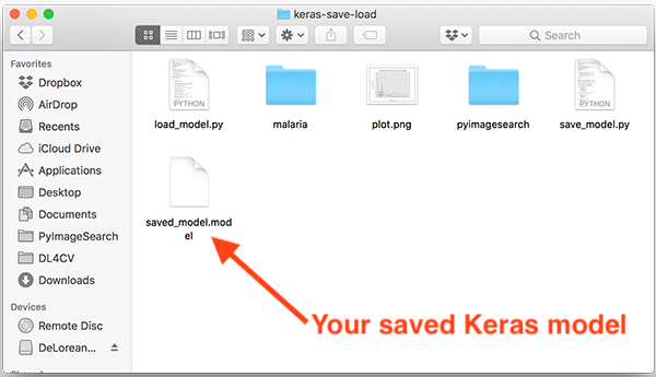 Figure 3: Our Keras model is now residing on disk. Saving Keras models is quite easy via the Keras API.
The saved_model.model file is your actual saved Keras model.
You will learn how to load your saved Keras model from disk in the next section.
Loading a model with Keras
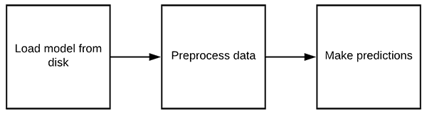
Figure 4: The process of loading a Keras model from disk and putting it to use to make predictions. Don’t forget to preprocess your data in the same manner as during training!
Now that we’ve learned how to save a Keras model to disk, the next step is to load the Keras model so we can use it for making classifications. Open up your load_model.py script and let’s get started:
| 1234567891011121314151617 | # import the necessary packagesfrom keras.preprocessing.image import img_to_arrayfrom keras.models import load_modelfrom imutils import build_montagesfrom imutils import pathsimport numpy as npimport argparseimport randomimport cv2 # construct the argument parser and parse the argumentsap = argparse.ArgumentParser()ap.add_argument(“-i”, “–images”, required=True, help=”path to out input directory of images”)ap.add_argument(“-m”, “–model”, required=True, help=”path to pre-trained model”)args = vars(ap.parse_args()) |
2
4
6
8
10
12
14
16
from keras.preprocessing.image import img_to_array
from imutils import build_montages
import numpy as np
import random
ap = argparse.ArgumentParser()
help=”path to out input directory of images”)
help=”path to pre-trained model”)
We import our required packages on Lines 2-10. Most notably we need load_model in order to load our model from disk and put it to use.
Our two command line arguments are parsed on Lines 12-17:
–images : The path to the images we’d like to make predictions with.
–model : The path to the model we just saved previously.
Again, these lines don’t need to change. When you enter the command in your terminal you’ll provide values for both –images and –model .
The next step is to load our Keras model from disk:
| # load the pre-trained networkprint(“[INFO] loading pre-trained network…“)model = load_model(args[“model”]) |
print(“[INFO] loading pre-trained network…”)
On Line 21, to load our Keras model , we call load_model , providing the path to the model itself (contained within our parsed args dictionary).
Given the model , we can now make predictions with it. But first we’ll need some images to work with and a place to put our results:
| # grab all image paths in the input directory and randomly sample themimagePaths = list(paths.list_images(args[“images”]))random.shuffle(imagePaths)imagePaths = imagePaths[:16] # initialize our list of resultsresults = [] |
imagePaths = list(paths.list_images(args[“images”]))
imagePaths = imagePaths[:16]
initialize our list of results
On Lines 24-26, we grab a random selection of testing image paths.
Line 29initializes an empty list to hold the results .
Let’s loop over each of our imagePaths :
| # loop over our sampled image pathsfor p in imagePaths: # load our original input image orig = cv2.imread(p) # pre-process our image by converting it from BGR to RGB channel # ordering (since our Keras mdoel was trained on RGB ordering), # resize it to 64x64 pixels, and then scale the pixel intensities # to the range [0, 1] image = cv2.cvtColor(orig, cv2.COLOR_BGR2RGB) image = cv2.resize(image, (64, 64)) image = image.astype(“float”) / 255.0 |
for p in imagePaths:
orig = cv2.imread(p)
# pre-process our image by converting it from BGR to RGB channel
# resize it to 64x64 pixels, and then scale the pixel intensities
image = cv2.cvtColor(orig, cv2.COLOR_BGR2RGB)
image = image.astype(“float”) / 255.0
On Line 32 we begin looping over our imagePaths .
We begin the loop by loading our image from disk (Line 34) and preprocessing it (Lines 40-42). These preprocessing steps should be identical to those taken in our training script. As you can see, we’ve converted the images from BGR to RGB channel ordering, resized to 64×64 pixels, and scaled to the range [0, 1].
A common mistake I see new deep learning practitioners make is failing to preprocess new images in the same manner as their training images.
Moving on, let’s make a prediction an image each iteration of the loop:
| 4445464748495051525354555657585960616263646566 | # order channel dimensions (channels-first or channels-last) # depending on our Keras backend, then add a batch dimension to # the image image = img_to_array(image) image = np.expand_dims(image, axis=0) # make predictions on the input image pred = model.predict(image) pred = pred.argmax(axis=1)[0] # an index of zero is the ‘parasitized’ label while an index of # one is the ‘uninfected’ label label = “Parasitized” if pred == 0 else “Uninfected” color = (0, 0, 255) if pred == 0 else (0, 255, 0) # resize our original input (so we can better visualize it) and # then draw the label on the image orig = cv2.resize(orig, (128, 128)) cv2.putText(orig, label, (3, 20), cv2.FONT_HERSHEY_SIMPLEX, 0.5, color, 2) # add the output image to our list of results results.append(orig) |
45
47
49
51
53
55
57
59
61
63
65
# depending on our Keras backend, then add a batch dimension to
image = img_to_array(image)
pred = model.predict(image)
# one is the ‘uninfected’ label
color = (0, 0, 255) if pred == 0 else (0, 255, 0)
# resize our original input (so we can better visualize it) and
orig = cv2.resize(orig, (128, 128))
color, 2)
# add the output image to our list of results
In this block we:
Handle channel ordering (Line 47). The TensorFlow backend default is “channels_first” , but don’t forget that Keras supports alternative backends as well.
- Create a batch to send through the network by adding a dimension to the volume (Line 48). We’re just sending one image through the network at a time, but the additional dimension is critical.
Pass image through ResNet model (Line 51), obtaining a prediction. We take the index of the max prediction (either “Parasitized” or “Uninfected” ) on Line 52.
- Then we create a colored label and draw it on the original image (Lines 56-63).
Finally, we append the annotated orig image to results .
To visualize our results let’s create a montage and display it on the screen:
| # create a montage using 128x128 “tiles” with 4 rows and 4 columnsmontage = build_montages(results, (128, 128), (4, 4))[0] # show the output montagecv2.imshow(“Results”, montage)cv2.waitKey(0) |
montage = build_montages(results, (128, 128), (4, 4))[0]
show the output montage
cv2.waitKey(0)
A montage of results is built on Line 69. Our montage is a 4×4 grid of images to accommodate the 16 random testing images we grabbed earlier on. Learn how this function works in my blog post, Montages with OpenCV.
The montage will be displayed until any key is pressed (Lines 72 and 73).
To see our script in action make sure you use the “Downloads” section of the tutorial to download the source code and dataset of images.
From there, open up a terminal and execute the following command:
| $ python load_model.py –images malaria/testing –model saved_model.modelUsing TensorFlow backend.[INFO] loading pre-trained network… |
Using TensorFlow backend.
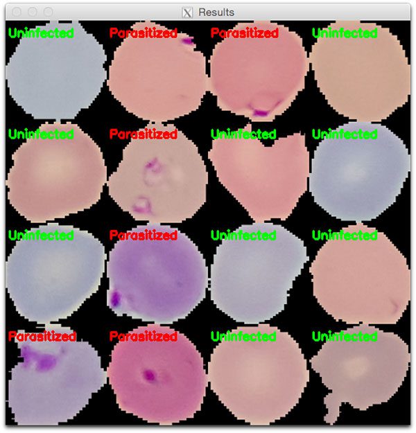 Figure 5: A montage of cells either “Parasitized” or “Uninfected” with Malaria. In today’s blog post we saved a ResNet deep learning model to disk and then loaded it with a separate script to make these predictions.
Here you can see that we have:
Provided the path to our testing images ( –images malaria/testing ) as well as the model already residing on disk ( –model saved_model.model ) via command line argument
-
Loaded our Keras model from disk
-
Preprocessed our input images
-
Classified each of the example images
-
Constructed an output visualization of our classifications (Figure 5)
This process was made possible due to the fact we were able to save our Keras model from disk in the training script and then load the Keras model from disk in a separate script.
Summary
In today’s tutorial you learned:
-
How to train a Keras model on a dataset
-
How to serialize and save your Keras model to disk
-
How to load your saved Keras model from a separate Python script
-
How to classify new input images using your loaded Keras model
You can use the Python scripts covered in today’s tutorial as templates when training, saving, and loading your own Keras models.
I hope you enjoyed today’s blog post!
To download the source code to today’s tutorial, and be notified when future blog posts are published here on PyImageSearch, just enter your email address in the form below!