Self Avoiding Walks

This week, I’m going to talk about space filling self-avoiding walks.

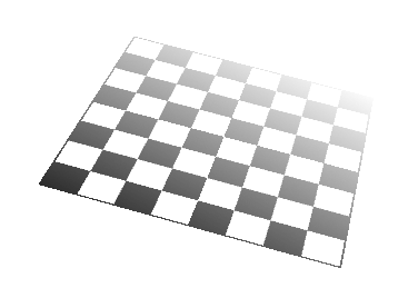
Imagine you had a chess board, and you started on one square. If you were allowed to only move one square at a time, horizontally or vertically (but not diagonally) to a previously un-visited square, is it possible to find a tour that visits all the squares on the board?

Is it always possible? Does it depend on where you start? How does this change with the size of the grid?

Here is an example for an 8x8 grid (starting from where a bishop would start a game).

Try it out

Here’s a little application for you to try it out yourself. Using the buttons on the right you can define the grid size. Each time the board is redrawn the start seed moves to a random position (You can force this by clicking the Reset button). Click on the grid to extend the path, and use Undo to, recursively, remove the last step if you back yourself into a corner.

Did you find any patterns?

Hamiltonian Paths

1x1

Returning to our initial problem, let’s start by looking at a 1x1 grid. This is trivial. There’s only one path!

2x2

This is also trivial. There are two solutions (no matter where we start). Our first move can be either horizontal, or vertical (the only two choices); after that, the other moves are automatic.

3x3

This is the first, non-trivial, problem. If we start at one of the corners, there are just eight possible solutions. (It does not matter which corner, as the solutions are symmetrical both in rotation and reflection).

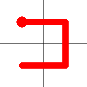
Tours that start at a corner are called Greek Key Tours (presumably in reference to the popular tiling pattern?).

If we start in the center, there are also eight solutions.

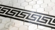
However, if we start at one of the edge pieces, there is no solution. Why is this? Well, the checkerboard pattern gives us a strong clue. If we shade the board alternating black and white we can see that a move from a square changes the parity of the color. If we were on a black square, a move will change us to a white square, and vice-versa. Because of the odd sized grid, there are an odd number of squares in total (in the example here, there is one more white square than black squares).

The only way to toggle, alternately, between colors is to start on a white square, and finish on a white square. There can be no solution if we start on a black square.

4x4

There are an equal number of black and white squares on an even sized square board, so there are no parity restrictions. There are solutions from every starting position. However, there are the most solutions when the route starts in a corner (The Greek Key Tour). Here is a count of all the possible solutions based on their starting condition. It’s should be no surprise at the symmetry.

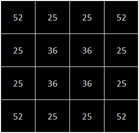
Here are the 52 solutions starting at a corner space:

Here are the 25 solutions starting at one of the edge locations:

Here are the 36 solutions possible from one of the four center locations:

5x5

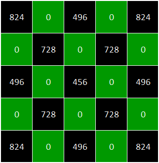
For 5x5 we’re back to having parity restrictions on every other space (as we have for all odd-sized boards). Again, the Greek Key Tour offers the highest number of possible solutions at 824.

Here is a count of all the possible solutions based on their starting condition. There are no solutions starting from any green square.

Here is one example solution:

6x6

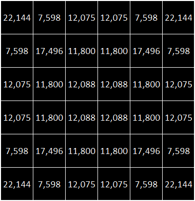
The number of solutions is starting to increase rapidly now. Here are the enumerations of possible solutions based on starting position. The number of Greek Key solutions is 22,144. As this is an even grid, there are solutions from every possible starting space.

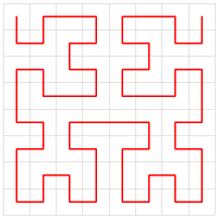
Here is one example solution:

7x7 and beyond …

I’m not sure if a formula has been derived for determining the number of Greek Key solutions based on arbitrary grid sizes, but here are the number of solutions for the first fifteen square grids:

Grid	Number of Greek Key Tour Solutions	——
1	1
2	2
3	8
4	52
5	824
6	22,144
7	1,510,446
8	180,160,012
9	54,986,690,944
10	29,805,993,260,994
11	41,433,610,713,353,366
12	103,271,401,574,007,978,038
13	660,340,630,211,753,942,588,170
14	7,618,229,614,763,015,717,175,450,784
15	225,419,381,425,094,248,494,363,948,728,158

Space Filing Curves

Generating Hamiltonian Paths

Instead of enumerating all possible permutations, another alternative is to randomly generate them. One popular way to do this is to use an algorithm called the backbite algorithm.

We start with a non-random Hamiltonian Path, such as a basic, easy to make, zig-zag pattern. Then, random changes are made to morph this into a different path. Using the procedures described below it ensures that the next generated graph is also a Hamiltonian path, and the constraints maintained.

Algorithm

• Select either of the two end points on the current graph.

• Select, at random, one of the neighbor vertices of this end point that is not the one connected to the current point. (If the chosen vertex happens to be the opposite endpoint, add an edge to it and remove the edge that it was connected to originally).

• This creates a loop, and the selected node now has a valency of three. (One link is the edge just created. One will lead to the opposite end of the graph, and the third loops back to itself).

• The one that loops back to itself should be removed. This is the backbite.

The resulting graph remains Hamiltonian. The randomization can be repeated as often as desired.

Example

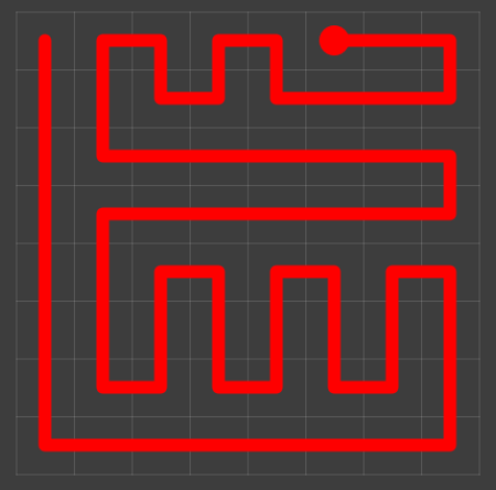
Here’s a walk-through example.

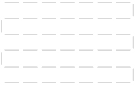
Considering the following path, which is already a Hamiltonian Path.

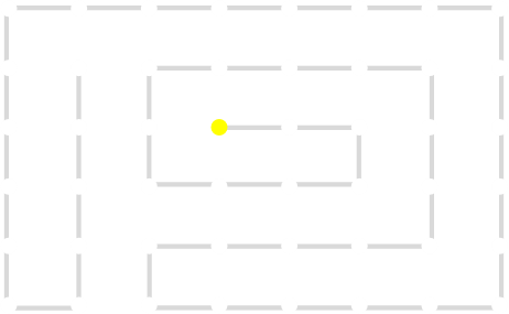
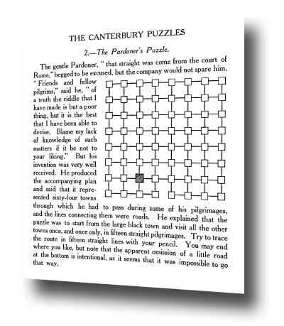
One of the end nodes is selected at random. This is shown in yellow.

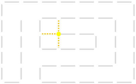
A new link is to be added. Connections to the nearest neighbors are considering (other than the the link that is already present at this node). The possible new links are shown in dotted orange.

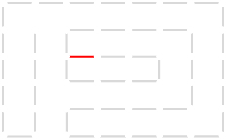
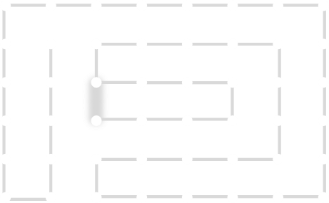
One of these candidates is selected at random and added to to the graph. This is shown in red. The addition of this new edge creates a loop in the graph.

Adding this link also creates a node with a valency of three. The newly created link remains, and we need to determine which of the other two links to break. This is done by propagating along each of the other two links. One of the these paths will take us to the other end-node of the graph, and the other will loop back on itself.

The link that forms the loop is deleted.

This is the backbite.

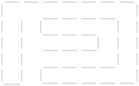
And the final result is a new Hamiltonian Path!