By Dipanjan Sarkar, Intel

Introduction
This article is a continuation in my series of articles aimed at ‘Explainable Artificial Intelligence (XAI)’. If you haven’t checked out the first article, I would definitely recommend you to take a quick glance at ‘Part I — The Importance of Human Interpretable Machine Learning’ which covers the what and why of human interpretable machine learning and the need and importance of model interpretation along with its scope and criteria. In this article, we will be picking up from where we left off and expand further into the criteria of machine learning model interpretation methods and explore techniques for interpretation based on scope. The aim of this article is to give you a good understanding of existing, traditional model interpretation methods, their limitations and challenges. We will also cover the classic model accuracy vs. model interpretability trade-off and finally take a look at the major strategies for model interpretation.
Briefly, we will be covering the following aspects in this article.
Traditional Techniques for Model Interpretation Challenges and Limitations of Traditional Techniques The Accuracy vs. Interpretability trade-off Model Interpretation Techniques
This should get us set and ready for the detailed hands-on guide to model interpretation coming in Part 3, so stay tuned!
Traditional Techniques for Model Interpretation
Model interpretation at heart, is to find out ways to understand model decision making policies better. This is to enable fairness, accountability and transparency which will give humans enough confidence to use these models in real-world problems which a lot of impact to business and society. Hence, there are techniques which have existed for a long time now, which can be used to understand and interpret models in a better way. These can be grouped under the following two major categories.
Let’s briefly take a more detailed look at these techniques.
Exploratory Analysis and Visualization
The idea of exploratory analysis is not something entirely new. For years now, data visualization has been one of the most effective tools for getting latent insights from data. Some of these techniques can help us in identifying key features and meaningful representations from our data which can give an indication of what might be influential for a model to take decisions in a human-interpretable form.
Dimensionality reduction techniques are very useful here since often we deal with a very large feature space (curse of dimensionality) and reducing the feature space helps us visualize and see what might be influencing a model to take specific decisions. Some of these techniques are as follows.
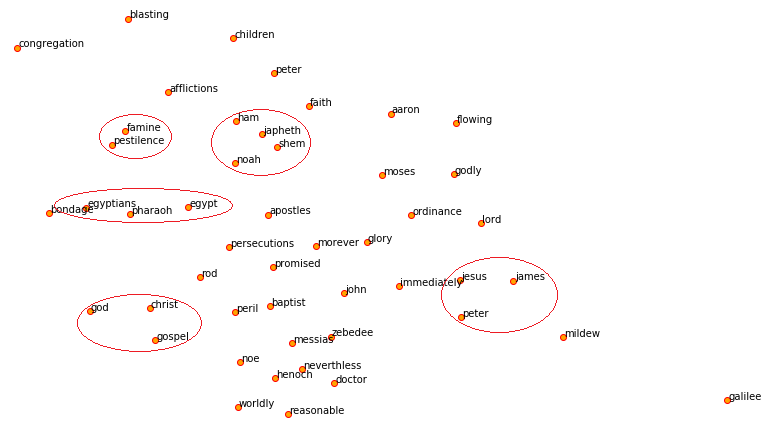
An example of this in a real-world problem could be trying to visualize which text features could be influential in a model by checking their semantic similarity using word embeddings and visualizing the same using t-SNE as depicted below.
You can also use t-SNE to visualize the famous MNIST hand-written digits dataset as depicted in the following figure.
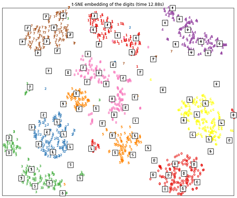 Visualizing MNIST data using t-SNE using sklearn. Image courtesy of Pramit Choudhary and the Datascience.com team.
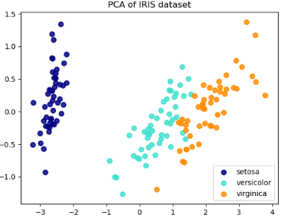
Another example is visualizing the famous IRIS dataset by leveraging PCA for dimension reduction as depicted in the following figure.
Besides visualizing data and features, certain more intuitive and interpretable models like decision trees help us in visualizing how exactly it might take a certain decision. A sample tree is depicted below which helps us visualize the exact rules in a human-interpretable manner.
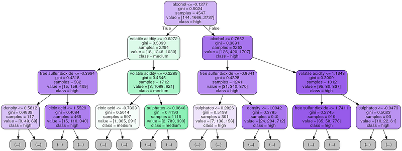
However, like we discussed we may not get these rules for other models which are not as interpretable as tree based models. Also huge decision trees always become very difficult to visualize and interpret.
Model Performance Evaluation Metrics
Model performance evaluation is a key step in any data science lifecycle for choosing the best model. This enables us to see how well our models are performing, compare various performance metrics across models and choose the best models. This also enables us to tune and optimize hyper-parametersin a model to obtain a model which gives the best performance on the data we are dealing with. Typically there exist certain standard evaluation metrics based on the type of problem we are dealing with.
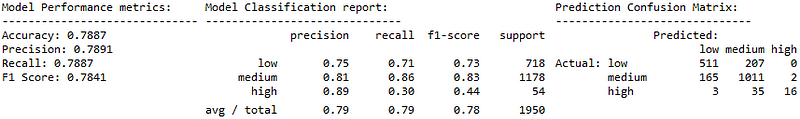
Supervised Learning — Classification: For classification problems, our main objective is to predict a discrete categorical response variable. The confusion matrix is extremely useful here from which we can derive a whole bunch of useful metrics including accuracy, precision, recall, F1-Score as depicted in the following example.
Besides these metrics, we can also use some other techniques like the ROC curve and the AUC score as depicted in a wine-quality prediction system in the following figure.
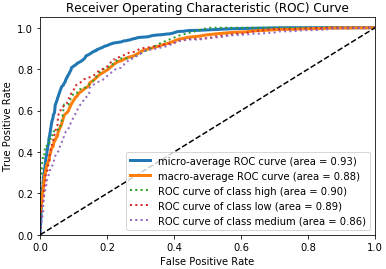
The area under the ROC curve is a very popular technique to objectively evaluate the performance of a classifier. Here we typically try to balance the True Positive Rate (TPR) and the False Positive Rate (FPR). The above figure tells us that the AUC score for a wine of class **‘high’** is **0.9** which means that the model’s probability of assigning a higher score to a wine of class **‘high’**(positive class) than to class **NOT ‘high’**which is either **‘medium’** or **‘low’**(negative class) is 90%. At times, the results may be misleading and difficult to interpret if the ROC curves cross(Source: Measuring classifier performance: a coherent alternative to the area under the ROC curve).
Limitations of Traditional Techniques and Motivation for Better Model Interpretation
The techniques we discussed in the previous techniques are definitely helpful in trying to understand more about our data, features as well as which models might be effective. However, they are quite limiting in terms of trying to discern human-interpretable ways of how a model works. In any data science problem, we usually build a model on a stationary dataset and get our objective function (optimized loss function) which is usually deployed when it meets certain criteria based on model performance and business requirements. Usually we leverage the above techniques of exploratory analysis and evaluation metrics for deciding the overall model performance on our data. However, in the real-world, a model’s performance often decreases and plateaus over time after deployment due to variability in data features, added constraints and noise. This might include things like changes in the environment, changes in features as well as added constraints. Hence simply re-training a model on the same feature set will not be sufficient and we need to constantly check for how important features are in deciding model predictions and how well they might be working on new data points.
For example, an intrusion detection system(IDS), a cyber-security application, is prone to evasion attacks where an attacker may use adversarial inputs to beat the secure system (note: adversarial inputs are examples that are intentionally engineered by an attacker to trick the machine learning model to make false predictions). The model’s objective function in such cases may act as a weak surrogate to the real-world objectives. A better interpretation might be needed to identify the blind spots in the algorithms to build a secure and safe model by fixing the training data set prone to adversarial attacks (for further reading, see Moosavi-Dezfooli, et al., 2016, DeepFool and Goodfellow, et al., 2015, Explaining and harnessing adversarial examples).
 Source: https://medium.com/@jrodthoughts/using-adversarial-attacks-to-make-your-deep-learning-model-look-stupid-24fb872f06fd
Besides, often bias exists in models due to the nature of data we are dealing with like in a rare-class prediction problem (fraud or intrusion detection). Metrics don’t help us justify the true story of a model’s prediction decisions. Also these traditional forms of model interpretation might be easy for a data scientist to understand but since they are inherently theoretical and often mathematical, there is a substantial gap in trying to explain these to (non-technical) business stakeholders and trying to decide the success criteria of a project based on these metrics alone. Just telling the business, “I have a model with 90% accuracy” is not sufficient information for them to start trusting the model when deployed in the real world. We need human-interpretable interpretations (HII) of a model’s decision policies which could be explained with proper and intuitive inputs and outputs. This would enable insightful information to be easily shared with peers (analysts, managers, data scientists, data engineers). Using such forms of explanations, which could be explained based on inputs and outputs, might help facilitate better communication and collaboration, enabling businesses to make more confident decisions (e.g., risk assessment/audit risk analysis in financial institutions).
To reiterate, we define model interpretation (new approaches) as being able to account for fairness (unbiasedness/non-discriminative), accountability(reliable results), and transparency (being able to query and validate predictive decisions) of a predictive model — currently in regard to supervised learning problems.