Deep Learning and Medical Image Analysis with Keras

In this tutorial, you will learn how to apply deep learning to perform medical image analysis. Specifically, you will discover how to use the Keras deep learning library to automatically analyze medical images for malaria testing.

Such a deep learning + medical imaging system can help reduce the 400,000+ deaths per year caused by malaria.

Today’s tutorial was inspired by two sources. The first one was from PyImageSearch reader, Kali, who wrote in two weeks ago and asked:

Hi Adrian, thanks so much for your tutorials. They’ve helped me as I’ve been studying deep learning. I live in an area of Africa that is prone to disease, especially malaria. I’d like to be able to apply computer vision to help reduce malaria outbreaks. Do you have any tutorials on medical imaging? I would really appreciate it if you wrote one. Your knowledge can help me which can help me help others too.

Soon after I saw Kali’s email I stumbled on a really interesting article from Dr. Johnson Thomas, a practicing endocrinologist, who provided a great benchmark summarizing the work of the United States National Institutes of Health (NIH) used to build an automatic malaria classification system using deep learning.

Johnson compared NIH’s approach (~95.9% accurate) with two models he personally trained on the same malaria dataset (94.23% and 97.1% accurate, respectively).

That got me thinking — how could I contribute to deep learning and medical image analysis? How could I help the fight against malaria? And how could I help readers like Kali get their start in medical image analysis?

To make the project even more interesting, I decided I was going to minimize the amount of custom code I was going to write.

Time is of the essence in disease outbreaks — if we can utilize pre-trained models or existing code, fantastic. We’ll be able to help doctors and clinicians working in the field that much faster.

Therefore, I decided to:

1. Utilize models and code examples I had already created for my book, Deep Learning for Computer Vision with Python.

2. And demonstrate how you can take this knowledge and easily apply it to your own projects (including deep learning and medical imaging).

Over 75%+ of today’s code comes directly from my book with only a few modifications, enabling us to quickly train a deep learning model capable of replicating NIH’s work at a fraction of both (1) training time and (2) model size.

To learn how to apply deep learning to medical image analysis (and not to mention, help fight the malaria endemic), just keep reading.

Deep Learning and Medical Image Analysis with Keras

In the first part of this tutorial, we’ll discuss how deep learning and medical imaging can be applied to the malaria endemic.

From there we’ll explore our malaria database which contains blood smear images that fall into one of two classes: positive for malaria or negative for malaria.

After we’ve explored the database we’ll briefly review the directory structure for today’s project.

We’ll then train a deep learning model on our medical images to predict if a given patient’s blood smear is positive for malaria or not.

Finally, we’ll review our results.

Deep learning, medical imaging, and the malaria endemic

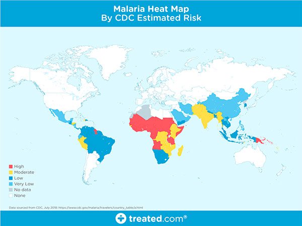
Figure 1: A world map of areas currently affected by malaria (source).

Malaria is an infectious disease that causes over 400,000 deaths per year.

Malaria is a true endemic in some areas of the world, meaning that the disease is regularly found in the region.

In other areas of the world, malaria is an epidemic — it’s widespread in the area but not yet at endemic proportions.

Yet in other areas of the world malaria is rarely, if ever, found at all.

So, what makes some areas of the world more susceptible to malaria while others are totally malaria free?

There are many components that make an area susceptible to an infectious disease outbreak. We’ll the primary constituents below.

Poverty level

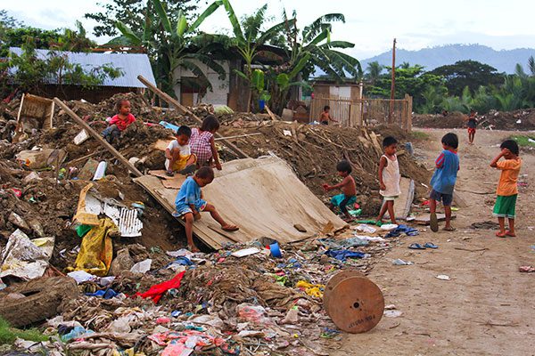
Figure 2: There is a correlation between areas of poverty and areas affected by malaria.

When assessing the risk of infectious disease outbreak we typically examine how many people in the population or at or below poverty levels.

The higher the poverty level, the higher the risk of infectious disease, although some researchers will say the opposite — that malaria causes poverty.

Whichever the cause we all can agree there is a correlation between the two.

Access to proper healthcare

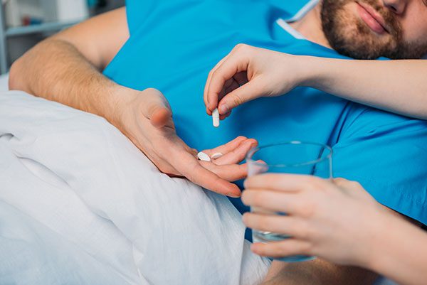
Figure 3: Areas lacking access to proper and modern healthcare can be affected by infectious disease.

Regions of the world that are below poverty levels most likely do not have access to proper healthcare.

Without good healthcare, proper treatment, and if necessary, quarantine, infectious diseases can spread quickly.

War and government

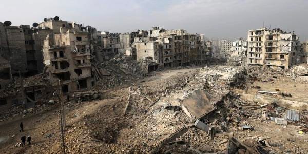
Figure 4: Areas of the world experiencing war have higher poverty levels and lower access to proper healthcare; thus, infectious disease outbreaks are common in these areas (source).

Is the area war-torn?

Is the government corrupt?

Is there in-fighting amongst the states or regions of a country?

Not surprisingly, an area of the world that either has a corrupt government or is experiencing civil war will also have higher poverty levels and lower access to proper healthcare.

Furthermore, if may be impossible for a corrupt government to provide emergency medical treatment or issue proper quarantines during a massive outbreak.

Disease transmission vectors

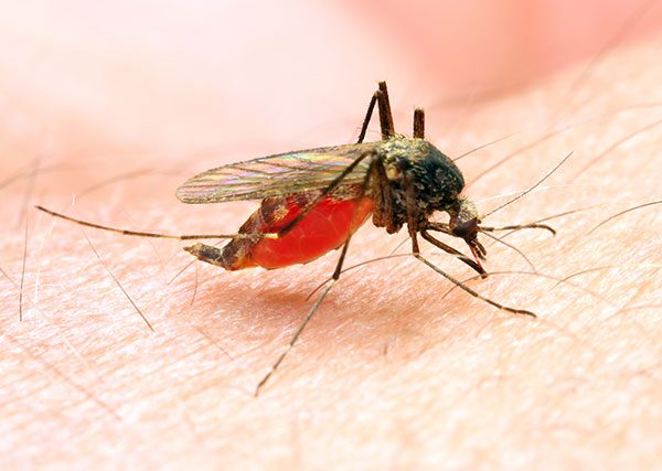
Figure 5: Disease vectors such as mosquitos can carry infectious diseases like malaria.

A disease vector is an agent that carries the disease and spreads it to other organisms. Mosquitoes are notorious for carrying malaria.

Once infected, a human can also be a vector and can spread malaria through blood transfusions, organ transplants, sharing needles/syringes, etc.

Furthermore, warmer climates of the world allow mosquitoes to flourish, further spreading disease.

Without proper healthcare, these infectious diseases can lead to endemic proportions.

How can we test for malaria?

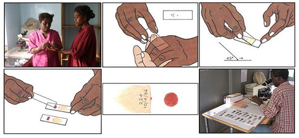
Figure 6: Two methods of testing for malaria include (1) blood smears, and (2) antigen testing (i.e. rapid tests). These are the two common means of testing for malaria that are most often discussed and used (source).

I want to start this section by saying I am not a clinician nor an infectious disease expert.

I will do my best to provide an extremely brief review of malaria testing.

If you want a more detailed review of how malaria is tested and diagnosed, please refer to Carlos Atico Ariza’s excellent article (who deserves all the credit for Figure 6 above).

There are a handful of methods to test for malaria, but the two I most frequently have read about include:

1. Blood smears

2. Antigen testing (i.e., rapid tests

The blood smear process can be visualized in Figure 6 above:

1. First, a blood sample is taken from a patient and then placed on a slide.

2. The sample is stained with a contrasting agent to help highlight malaria parasites in red blood cells

3. A clinician then examines the slide under a microscope and manually counts the number of red blood cells that are infected.

According to the official WHO malaria parasite counting protocol, a clinician may have to manually count up to 5,000 cells, an extremely tedious and time-consuming process.

In order to help make malaria testing a faster process in the field, scientists and researchers have developed antigen tests for Rapid Diagnosis Testing (RDT).

An example of an RDT device used for malaria testing can be seen below:

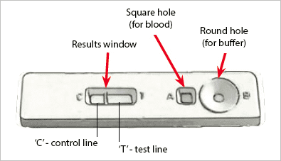
Figure 7: An antigen test classified as Rapid Diagnosis Testing (RDT) involves a small device that allows a blood sample and buffer to be added. The device performs the test and provides the results. These devices are fast to report a result, but they are also significantly less accurate (source).

Here you can see a small device that allows both a blood sample and a buffer to be added.

Internally, the device performs the test and provides the results.

While RDTs are significantly faster than cell counting they are also much less accurate.

An ideal solution would, therefore, need to combine the speed of RDTs with the accuracy of microscopy.

Note: A big thank you to Carlos Atico Azira’s excellent write up on malaria diagnosis. Please refer to his article for more information on malaria, how it spreads, and methods for automatically testing for malaria.

NIH’s proposed deep learning solution

In 2018, Rajaraman et al. published a paper entitled Pre-trained convolutional neural networks as feature extractors toward improved parasite detection in thin blood smear images.

In their work Rajaraman et al. utilized six pre-trained Convolutional Neural Networks, including:

• AlexNet

• VGG-16

• ResNet-50

• Xception

• DenseNet-121

• A customized model they created

Feature extraction and subsequent training took a little over 24 hours and obtained an impressive 95.9% accuracy.

The problem here is the number of models being utilized — it’s inefficient.

Imagine being a field worker in a remote location with a device pre-loaded with these models for malaria classification.

Such a model would have to be some combination:

1. Battery operated

2. Require a power (i.e., plugged into the wall)

3. Be connected to the cloud (requiring an internet connection)

Let’s further break down the problem:

1. In remote, poverty-stricken areas of the world, it may be impossible to find a reliable power source — battery operated would be better, allowing for charging whenever power is found.

2. But if you go with a battery operated device you’ll have less computational horsepower — trying to run all six of those models would drain your battery that much faster.

3. So, if battery life is a concern we should utilize the cloud — but if you use the cloud you’re dependent on a reliable internet connection which you may or may not have.

I’m obviously highlighting the worst-case scenarios for each item. You could certainly apply a bit of engineering and create a smartphone app that will push medical images to the cloud if an internet connection is available and then falls back to using the models stored locally on the phone, but I think you get my point.

Overall, it would be desirable to:

1. Obtain the same level of accuracy as NIH

2. With a smaller, more computationally efficient model

3. That can be easily deployed to edge and Internet of Things (IoT) devices

In the rest of today’s tutorial, I’ll show you how to do exactly that.

Our malaria database

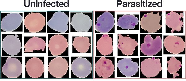
Figure 8: A subset of the Malaria Dataset provided by the National Institute of Health (NIH). We will use this dataset to develop a deep learning medical imaging classification model with Python, OpenCV, and Keras.

The malaria dataset we will be using in today’s deep learning and medical image analysis tutorial is the exact same dataset that Rajaraman et al. used in their 2018 publication.

The dataset itself can be found on the official NIH webpage:

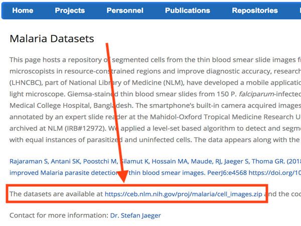
Figure 9: The National Institute of Health (NIH) has made their Malaria Dataset available to the public on their website.

You’ll want to go ahead and download the cell_images.zip  file on to your local machine if you’re following along with the tutorial.

The dataset consists of 27,588 images belonging to two separate classes:

1. Parasitized: Implying that the region contains malaria.

2. Uninfected: Meaning there is no evidence of malaria in the region.

The number of images per class is equally distributed with 13,794 images per each respective class.

Install necessary software

The software to run today’s scripts is very easy to install. To set everything up, you’ll use pip , virtualenv , and virtualenvwrapper . Be sure to follow the link in the Keras bullet below, first.

To run today’s code you will need:

• Keras: Keras is my favorite deep learning framework. Read and follow my tutorial, Installing Keras with the TensorFlow backend.

• NumPy & Scikit-learn: If you followed the Keras install instructions linked directly above, these packages for numerical processing and machine learning will be installed.

Matplotlib: The most popular plotting tool for Python. Once you have your Keras environment ready and active, you can install via pip install matplotlib . imutils: My personal package of image processing and deep learning convenience functions can be installed via pip install –upgrade imutils .

Project structure

Be sure to grab the “Downloads” for the post. The dataset isn’t included, but the instructions in this section will show you how to download it as well.

First, change directories and unzip the files:

$ cd /path/where/you/downloaded/the/files$ unzip dl-medical-imaging.zip

$ unzip dl-medical-imaging.zip

Then change directory into the project folder and create a malaria/  directory + cd  into it:

$ cd dl-medical-imaging$ mkdir malaria$ cd malaria

$ mkdir malaria

Next, download the dataset (into the dl-medical-imaging/malaria/  directory that you should currently be “in”):

$ wget https://ceb.nlm.nih.gov/proj/malaria/cell_images.zip$ unzip cell_images.zip

$ unzip cell_images.zip

If you don’t have the tree  package, you’ll need it:

$ sudo apt-get install tree # for Ubuntu$ brew install tree # for macOS

$ brew install tree # for macOS

Now let’s switch back to the parent directory:

Finally, let’s inspect our project structure now using the tree command:

$ tree –dirsfirst –filelimit 10.├── malaria│   ├── cell_images.zip│   └── cell_images│   │   ├── Parasitized [13780 entries]│   │   └── Uninfected [13780 entries]├── pyimagesearch│   ├── init.py│   ├── config.py│   └── resnet.py├── build_dataset.py├── train_model.py└── plot.png 5 directories, 7 files

.

│   ├── cell_images.zip

│   │   ├── Parasitized [13780 entries]

├── pyimagesearch

│   ├── config.py

├── build_dataset.py

└── plot.png

5 directories, 7 files

The NIH malaria dataset is located in the malaria/  folder. The contents have been unzipped. The cell_images/  for training and testing are categorized as Parasitized/  or Uninfected/ .

The pyimagesearch  module is the pyimagesearch/  directory. I often get asked how to pip-install pyimagesearch. You can’t! It is simply included with the blog post “Downloads”. Today’s pyimagesearch  module includes:

config.py : A configuration file. I opted to use Python directly instead of YAML/JSON/XML/etc. Read the next section to find out why as we review the config file.

resnet.py : This file contains the exact ResNet model class included with Deep Learning for Computer Vision with Python. In my deep learning book, I demonstrated how to replicated the ResNet model from the 2015 ResNet academic publication, Deep Residual Learning for Image Recognition by He et al.; I also show how to train ResNet on CIFAR-10, Tiny ImageNet, and ImageNet, walking you through each of my experiments and which parameters I changed and why.

Today we’ll be reviewing two Python scripts:

build_dataset.py : This file will segment our malaria cell images dataset into training, validation, and testing sets.

train_model.py : In this script, we’ll employ Keras and our ResNet model to train a malaria classifier using our organized data.

But first, let’s start by reviewing the configuration file which both scripts will need!

Our configuration file

When working on larger deep learning projects I like to create a config.py  file to store all my constant variables.

I could use a JSON, YAML, or equivalent files as well, but it’s nice being able to introduce Python code directly into your configuration.

Let’s review the config.py  file now:

123456789101112131415161718192021

# import the necessary packagesimport os # initialize the path to the original input directory of imagesORIG_INPUT_DATASET = “malaria/cell_images” # initialize the base path to the new directory that will contain# our images after computing the training and testing splitBASE_PATH = “malaria” # derive the training, validation, and testing directoriesTRAIN_PATH = os.path.sep.join([BASE_PATH, “training”])VAL_PATH = os.path.sep.join([BASE_PATH, “validation”])TEST_PATH = os.path.sep.join([BASE_PATH, “testing”]) # define the amount of data that will be used trainingTRAIN_SPLIT = 0.8 # the amount of validation data will be a percentage of the# training dataVAL_SPLIT = 0.1

2

4

6

8

10

12

14

16

18

20

import os

initialize the path to the original input directory of images

 

our images after computing the training and testing split

 

TRAIN_PATH = os.path.sep.join([BASE_PATH, “training”])

TEST_PATH = os.path.sep.join([BASE_PATH, “testing”])

define the amount of data that will be used training

 

training data

Let’s review the configuration briefly where we:

• Define the path to the original dataset of cell images (Line 5).

• Set our dataset base path (Line 9).

Establish the paths to the output training, validation, and testing directories (Lines 12-14). The build_dataset.py  file will be responsible for creating the paths in your filesystem.

• Define our training/testing split where 80% of the data is for training and the remaining 20% will be for testing (Line 17).

• Set our validation split where, of that 80% for training, we’ll take 10% for validation (Line 21).

Now let’s build our dataset!

Building our deep learning + medical image dataset

Our malaria dataset does not have pre-split data for training, validation, and testing so we’ll need to perform the splitting ourselves.

To create our data splits we are going to use the build_dataset.py  script — this script will:

1. Grab the paths to all our example images and randomly shuffle them.

2. Split the images paths into the training, validation, and testing.

Create three new sub-directories in the malaria/  directory, namely training/ , validation/ , and testing/.

1. Automatically copy the images into their corresponding directories.

To see how the data split process is performed, open up build_dataset.py  and insert the following code:

# import the necessary packagesfrom pyimagesearch import configfrom imutils import pathsimport randomimport shutilimport os # grab the paths to all input images in the original input directory# and shuffle themimagePaths = list(paths.list_images(config.ORIG_INPUT_DATASET))random.seed(42)random.shuffle(imagePaths)

from pyimagesearch import config

import random

import os

grab the paths to all input images in the original input directory

imagePaths = list(paths.list_images(config.ORIG_INPUT_DATASET))

random.shuffle(imagePaths)

Our packages are imported on Lines 2-6. Take note that we’re importing our config  from pyimagesearch  and paths  from imutils .

On Lines 10-12, images from the malaria dataset are grabbed and shuffled.

Now let’s split our data:

# compute the training and testing spliti = int(len(imagePaths) * config.TRAIN_SPLIT)trainPaths = imagePaths[:i]testPaths = imagePaths[i:] # we’ll be using part of the training data for validationi = int(len(trainPaths) * config.VAL_SPLIT)valPaths = trainPaths[:i]trainPaths = trainPaths[i:]

i = int(len(imagePaths) * config.TRAIN_SPLIT)

testPaths = imagePaths[i:]

we’ll be using part of the training data for validation

valPaths = trainPaths[:i]

The lines in the above code block compute training and testing splits.

First, we compute the index of the train/test split (Line 15). Then using the index and a bit of array slicing, we split the data into trainPaths  and testPaths  (Lines 16 and 17).

Again, we compute the index of the training/validation split from trainPaths  (Line 20). Then we split the image paths into valPaths  and trainPaths  (Lines 21 and 22). Yes, trainPaths  are reassigned because as I stated in the previous section, “…of that 80% for training, we’ll take 10% for validation”.

Now that we have our image paths organized into their respective splits, let’s define the datasets we’ll be building:

# define the datasets that we’ll be buildingdatasets = [ (“training”, trainPaths, config.TRAIN_PATH), (“validation”, valPaths, config.VAL_PATH), (“testing”, testPaths, config.TEST_PATH)]

datasets = [

(“validation”, valPaths, config.VAL_PATH),

]

Here I’ve created a list of 3-tuples (called datasets ) containing:

1. The name of the split

2. The image paths for the split

3. The path to the output directory for the split

With this information, we can begin to loop over each of the datasets :

3132333435363738394041424344454647484950515253545556575859

# loop over the datasetsfor (dType, imagePaths, baseOutput) in datasets: # show which data split we are creating print(“[INFO] building ‘{}’ split”.format(dType))  # if the output base output directory does not exist, create it if not os.path.exists(baseOutput): print(“[INFO] ‘creating {}’ directory”.format(baseOutput)) os.makedirs(baseOutput)  # loop over the input image paths for inputPath in imagePaths: # extract the filename of the input image along with its # corresponding class label filename = inputPath.split(os.path.sep)[-1] label = inputPath.split(os.path.sep)[-2]  # build the path to the label directory labelPath = os.path.sep.join([baseOutput, label])  # if the label output directory does not exist, create it if not os.path.exists(labelPath): print(“[INFO] ‘creating {}’ directory”.format(labelPath)) os.makedirs(labelPath)  # construct the path to the destination image and then copy # the image itself p = os.path.sep.join([labelPath, filename]) shutil.copy2(inputPath, p)

32

34

36

38

40

42

44

46

48

50

52

54

56

58

for (dType, imagePaths, baseOutput) in datasets:

print(“[INFO] building ‘{}’ split”.format(dType))

# if the output base output directory does not exist, create it

print(“[INFO] ‘creating {}’ directory”.format(baseOutput))

 

for inputPath in imagePaths:

# corresponding class label

label = inputPath.split(os.path.sep)[-2]

# build the path to the label directory

 

if not os.path.exists(labelPath):

os.makedirs(labelPath)

# construct the path to the destination image and then copy

p = os.path.sep.join([labelPath, filename])

On Line 32 we begin to loop over dataset type, image paths, and output directory.

If the output directory does not exist, we create it (Lines 37-39).

Then we loop over the paths themselves beginning on Line 42. In the loop, we:

Extract the filename  + label  (Lines 45 and 46).

• Create the subdirectory if necessary (Lines 49-54).

• Copy the actual image file itself into the subdirectory (Lines 58 and 59).

---

To build your malaria dataset make sure you have (1) used the “Downloads” section of this guide to download the source code + project structure and (2) have properly downloaded the cell_images.zip  file from NIH’s website as well.

From there, open up a terminal and execute the following command:

$ python build_dataset.py[INFO] building ‘training’ split[INFO] ‘creating malaria/training’ directory[INFO] ‘creating malaria/training/Uninfected’ directory[INFO] ‘creating malaria/training/Parasitized’ directory[INFO] building ‘validation’ split[INFO] ‘creating malaria/validation’ directory[INFO] ‘creating malaria/validation/Uninfected’ directory[INFO] ‘creating malaria/validation/Parasitized’ directory[INFO] building ‘testing’ split[INFO] ‘creating malaria/testing’ directory[INFO] ‘creating malaria/testing/Uninfected’ directory[INFO] ‘creating malaria/testing/Parasitized’ directory

[INFO] building ‘training’ split

[INFO] ‘creating malaria/training/Uninfected’ directory

[INFO] building ‘validation’ split

[INFO] ‘creating malaria/validation/Uninfected’ directory

[INFO] building ‘testing’ split

[INFO] ‘creating malaria/testing/Uninfected’ directory

The script itself should only take a few seconds to create the directories and copy images, even on a modestly powered machine.

Inspecting the output of build_dataset.py  you can see that our data splits have been successfully created.

Let’s take a look at our project structure once more just for kicks:

12345678910111213141516171819202122232425

$ tree –dirsfirst –filelimit 10.├── malaria│   ├── cell_images│   │   ├── Parasitized [13780 entries]│   │   └── Uninfected [13780 entries]│   ├── testing│   │   ├── Parasitized [2726 entries]│   │   └── Uninfected [2786 entries]│   ├── training│   │   ├── Parasitized [9955 entries]│   │   └── Uninfected [9887 entries]│   ├── validation│   │   ├── Parasitized [1098 entries]│   │   └── Uninfected [1106 entries]│   └── cell_images.zip├── pyimagesearch│   ├── init.py│   ├── config.py│   └── resnet.py├── build_dataset.py├── train_model.py└── plot.png 15 directories, 9 files

2

4

6

8

10

12

14

16

18

20

22

24

.

│   ├── cell_images

│   │   └── Uninfected [13780 entries]

│   │   ├── Parasitized [2726 entries]

│   ├── training

│   │   └── Uninfected [9887 entries]

│   │   ├── Parasitized [1098 entries]

│   └── cell_images.zip

│   ├── init.py

│   └── resnet.py

├── train_model.py

 

Notice that the new directories have been created in the malaria/  folder and images have been copied into them.

Training a deep learning model for medical image analysis

Now that we’ve created our data splits, let’s go ahead and train our deep learning model for medical image analysis.

As I mentioned earlier in this tutorial, my goal is to reuse as much code as possible from chapters in my book, Deep Learning for Computer Vision with Python. In fact, upwards of 75%+ of the code is directly from the text and code examples.

Time is of the essence when it comes to medical image analysis, so the more we can lean on reliable, stable code the better.

As we’ll see, we’ll able to use this code to obtain 97% accuracy.

Let’s go ahead and get started.

Open up the train_model.py  script and insert the following code:

123456789101112131415161718192021

# set the matplotlib backend so figures can be saved in the backgroundimport matplotlibmatplotlib.use(“Agg”) # import the necessary packagesfrom keras.preprocessing.image import ImageDataGeneratorfrom keras.callbacks import LearningRateSchedulerfrom keras.optimizers import SGDfrom pyimagesearch.resnet import ResNetfrom pyimagesearch import configfrom sklearn.metrics import classification_reportfrom imutils import pathsimport matplotlib.pyplot as pltimport numpy as npimport argparse # construct the argument parser and parse the argumentsap = argparse.ArgumentParser()ap.add_argument(“-p”, “–plot”, type=str, default=”plot.png”, help=”path to output loss/accuracy plot”)args = vars(ap.parse_args())

2

4

6

8

10

12

14

16

18

20

import matplotlib

 

from keras.preprocessing.image import ImageDataGenerator

from keras.optimizers import SGD

from pyimagesearch import config

from imutils import paths

import numpy as np

 

ap = argparse.ArgumentParser()

help=”path to output loss/accuracy plot”)

Since you followed my instructions in the “Install necessary software” section, you should be ready to go with the**imports on Lines 2-15**.

We’re using keras  to train our medical image deep learning model, sklearn  to print a classification_report , grabbing paths  from our dataset, numpy  for numerical processing, and argparse  for command line argument parsing.

The tricky one is matplotlib . Since we’re saving our plot to disk (and in my case, on a headless machine) we need to use the “Agg”  backend (Line 3).

Line 9 imports my ResNet  architecture implementation.

We won’t be covering the ResNet architecture in this tutorial, but if you’re interested in learning more, be sure to refer to the official ResNet publication as well as Deep Learning for Computer Vision with Python where I review ResNet in detail.

We have a single command line argument that is parsed on Lines 18-21, –plot . By default, our plot will be placed in the current working directory and named plot.png . Alternatively, you can supply a different filename/path at the command line when you go to execute the program.

Now let’s set our training parameters and define our learning rate decay function:

232425262728293031323334353637383940

# define the total number of epochs to train for along with the# initial learning rate and batch sizeNUM_EPOCHS = 20INIT_LR = 1e-1BS = 32 def poly_decay(epoch): # initialize the maximum number of epochs, base learning rate, # and power of the polynomial maxEpochs = NUM_EPOCHS baseLR = INIT_LR power = 1.0  # compute the new learning rate based on polynomial decay alpha = baseLR * (1 - (epoch / float(maxEpochs))) ** power  # return the new learning rate return alpha

24

26

28

30

32

34

36

38

40

initial learning rate and batch size

INIT_LR = 1e-1

 

# initialize the maximum number of epochs, base learning rate,

maxEpochs = NUM_EPOCHS

power = 1.0

# compute the new learning rate based on polynomial decay

 

return alpha

On Lines 25-26, we define the number of epochs, initial learning rate, and batch size.

I found that training for  NUM_EPOCHS = 20  (training iterations) worked well. A BS = 32  (batch size) is adequate for most systems (CPU), but if you use a GPU you can increase this value to 64 or higher. Our INIT_LR = 1e-1  (initial learning rate) will decay according to the poly_decay  functions.

Our poly_dcay  function is defined on Lines 29-40. This function will help us decay our learning rate after each epoch. We’re setting power = 1.0  which effectively turns our polynomial decay into a linear decay. The magic happens in the decay equation on Line 37 the result of which is returned on Line 40.

Next, let’s grab the number of image paths in training, validation, and testing sets:

# determine the total number of image paths in training, validation,# and testing directoriestotalTrain = len(list(paths.list_images(config.TRAIN_PATH)))totalVal = len(list(paths.list_images(config.VAL_PATH)))totalTest = len(list(paths.list_images(config.TEST_PATH)))

and testing directories

totalVal = len(list(paths.list_images(config.VAL_PATH)))

We’ll need these quantity values to determine the total number of steps per epoch for the validation/testing process.

Let’s apply data augmentation (a process I nearly always recommend for every deep learning dataset):

48495051525354555657585960

# initialize the training training data augmentation objecttrainAug = ImageDataGenerator( rescale=1 / 255.0, rotation_range=20, zoom_range=0.05, width_shift_range=0.05, height_shift_range=0.05, shear_range=0.05, horizontal_flip=True, fill_mode=”nearest”) # initialize the validation (and testing) data augmentation objectvalAug = ImageDataGenerator(rescale=1 / 255.0)

49

51

53

55

57

59

trainAug = ImageDataGenerator(

rotation_range=20,

width_shift_range=0.05,

shear_range=0.05,

fill_mode=”nearest”)

initialize the validation (and testing) data augmentation object

On Lines 49-57 we initialize our ImageDataGenerator  which will be used to apply data augmentation by randomly shifting, translating, and flipping each training sample. I cover the concept of data augmentation in the Practitioner Bundle of Deep Learning for Computer Vision with Python.

The validation ImageDataGenerator will not perform any data augmentation (Line 60). Instead, it will simply rescale our pixel values to the range [0, 1], just like we have done for the training generator. Take note that we’ll be using the valAug  for both validation and testing.

Let’s initialize our training, validation, and testing generators:

6263646566676869707172737475767778798081828384858687

# initialize the training generatortrainGen = trainAug.flow_from_directory( config.TRAIN_PATH, class_mode=”categorical”, target_size=(64, 64), color_mode=”rgb”, shuffle=True, batch_size=BS) # initialize the validation generatorvalGen = valAug.flow_from_directory( config.VAL_PATH, class_mode=”categorical”, target_size=(64, 64), color_mode=”rgb”, shuffle=False, batch_size=BS) # initialize the testing generatortestGen = valAug.flow_from_directory( config.TEST_PATH, class_mode=”categorical”, target_size=(64, 64), color_mode=”rgb”, shuffle=False, batch_size=BS)

63

65

67

69

71

73

75

77

79

81

83

85

87

trainGen = trainAug.flow_from_directory(

class_mode=”categorical”,

color_mode=”rgb”,

batch_size=BS)

initialize the validation generator

config.VAL_PATH,

target_size=(64, 64),

shuffle=False,

 

testGen = valAug.flow_from_directory(

class_mode=”categorical”,

color_mode=”rgb”,

batch_size=BS)

In this block, we create the Keras generators used to load images from an input directory.

The flow_from_directory  function assumes:

1. There is a base input directory for the data split.

2. And inside that base input directory, there are N subdirectories, where each subdirectory corresponds to a class label.

Be sure to review the Keras preprocessing documentation as well as the parameters we’re feeding each generator above. Notably, we:

Set class_mode  equal to categorical  to ensure Keras performs one-hot encoding on the class labels. Resize all images to 64 x 64  pixels. Set our color_mode  to “rgb”  channel ordering.

• Shuffle image paths only for the training generator.

Use a batch size of BS = 32 .

Let’s initialize ResNet  and compile the model:

# initialize our ResNet model and compile itmodel = ResNet.build(64, 64, 3, 2, (3, 4, 6), (64, 128, 256, 512), reg=0.0005)opt = SGD(lr=INIT_LR, momentum=0.9)model.compile(loss=”binary_crossentropy”, optimizer=opt, metrics=[“accuracy”])

model = ResNet.build(64, 64, 3, 2, (3, 4, 6),

opt = SGD(lr=INIT_LR, momentum=0.9)

metrics=[“accuracy”])

On Line 90, we initialize ResNet:

Images are 64 x 64 x 3  (3-channel RGB images). We have a total of 2  classes. ResNet will perform (3, 4, 6)  stacking with (64, 128, 256, 512)  CONV layers, implying that:

The first CONV layer in ResNet, prior to reducing spatial dimensions, will have 64  total filters. Then we will stack 3  sets of residual modules. The three CONV layers in each residual module will learn 32, 32 and 128  CONV filters respectively. We then reduce spatial dimensions.

Again if you are interested in learning more about ResNet, including how to implement it from scratch, please refer to Deep Learning for Computer Vision with Python.

Line 92 initializes the SGD optimizer with the default initial learning of 1e-1  and a momentum term of 0.9 .

Lines 93 and 94 compile the actual model using binary_crossentropy  as our loss function (since we’re performing binary, 2-class classification). For greater than two classes we would use categorical_crossentropy .

We are now ready to train our model:

# define our set of callbacks and fit the modelcallbacks = [LearningRateScheduler(poly_decay)]H = model.fit_generator( trainGen, steps_per_epoch=totalTrain // BS, validation_data=valGen, validation_steps=totalVal // BS, epochs=NUM_EPOCHS, callbacks=callbacks)

callbacks = [LearningRateScheduler(poly_decay)]

trainGen,

validation_data=valGen,

epochs=NUM_EPOCHS,

On Line 97 we create our set of callbacks . Callbacks are executed at the end of each epoch. In our case we’re applying our poly_decay  LearningRateScheduler  to decay our learning rate after each epoch.

Our model.fit_generator  call on Lines 98-104 instructs our script to kick off our training process.

The trainGen  generator will automatically (1) load our images from disk and (2) parse the class labels from the image path.

Similarly, valGen  will do the same process, only for the validation data.

Let’s evaluate the results on our testing dataset:

106107108109110111112113114115116117118119

# reset the testing generator and then use our trained model to# make predictions on the dataprint(“[INFO] evaluating network…“)testGen.reset()predIdxs = model.predict_generator(testGen, steps=(totalTest // BS) + 1) # for each image in the testing set we need to find the index of the# label with corresponding largest predicted probabilitypredIdxs = np.argmax(predIdxs, axis=1) # show a nicely formatted classification reportprint(classification_report(testGen.classes, predIdxs, target_names=testGen.class_indices.keys()))

107

109

111

113

115

117

119

make predictions on the data

testGen.reset()

steps=(totalTest // BS) + 1)

for each image in the testing set we need to find the index of the

predIdxs = np.argmax(predIdxs, axis=1)

show a nicely formatted classification report

target_names=testGen.class_indices.keys()))

Now that model is trained we can evaluate on the test set.

Line 109 can technically be removed but anytime you use a Keras data generator you should get in the habit of resetting it prior to evaluation.

To evaluate our model we’ll make predictions on test data and subsequently find the label with the largest probability for each image in the test set (Lines 110-115).

Then we’ll print  our classification_report  in a readable format in the terminal (Lines 118 and 119).

Finally, we’ll plot our training data:

121122123124125126127128129130131132133

# plot the training loss and accuracyN = NUM_EPOCHSplt.style.use(“ggplot”)plt.figure()plt.plot(np.arange(0, N), H.history[“loss”], label=”train_loss”)plt.plot(np.arange(0, N), H.history[“val_loss”], label=”val_loss”)plt.plot(np.arange(0, N), H.history[“acc”], label=”train_acc”)plt.plot(np.arange(0, N), H.history[“val_acc”], label=”val_acc”)plt.title(“Training Loss and Accuracy on Dataset”)plt.xlabel(“Epoch #”)plt.ylabel(“Loss/Accuracy”)plt.legend(loc=”lower left”)plt.savefig(args[“plot”])

122

124

126

128

130

132

N = NUM_EPOCHS

plt.figure()

plt.plot(np.arange(0, N), H.history[“val_loss”], label=”val_loss”)

plt.plot(np.arange(0, N), H.history[“val_acc”], label=”val_acc”)

plt.xlabel(“Epoch #”)

plt.legend(loc=”lower left”)

Lines 122-132 generate an accuracy/loss plot for training and validation.

To save our plot to disk we call .savefig  (Line 133).

Medical image analysis results

Now that we’ve coded our training script, let’s go ahead and train our Keras deep learning model for medical image analysis.

If you haven’t yet, make sure you (1) use the “Downloads” section of today’s tutorial to grab the source code + project structure and (2) download the cell_images.zip  file from the official NIH malaria dataset page. I recommend following my project structure above.

From there, you can start training with the following command:

1234567891011121314151617181920212223242526

$ python train_model.pyFound 19842 images belonging to 2 classes.Found 2204 images belonging to 2 classes.Found 5512 images belonging to 2 classes….Epoch 1/50620/620 [==============================] - 67s - loss: 0.8723 - acc: 0.8459 - val_loss: 0.6020 - val_acc: 0.9508Epoch 2/50620/620 [==============================] - 66s - loss: 0.6017 - acc: 0.9424 - val_loss: 0.5285 - val_acc: 0.9576Epoch 3/50620/620 [==============================] - 65s - loss: 0.4834 - acc: 0.9525 - val_loss: 0.4210 - val_acc: 0.9609…Epoch 48/50620/620 [==============================] - 65s - loss: 0.1343 - acc: 0.9646 - val_loss: 0.1216 - val_acc: 0.9659Epoch 49/50620/620 [==============================] - 65s - loss: 0.1344 - acc: 0.9637 - val_loss: 0.1184 - val_acc: 0.9678Epoch 50/50620/620 [==============================] - 65s - loss: 0.1312 - acc: 0.9650 - val_loss: 0.1162 - val_acc: 0.9678[INFO] serializing network…[INFO] evaluating network…             precision    recall  f1-score   support Parasitized       0.97      0.97      0.97      2786 Uninfected       0.97      0.97      0.97      2726 avg / total       0.97      0.97      0.97      5512

2

4

6

8

10

12

14

16

18

20

22

24

26

Found 19842 images belonging to 2 classes.

Found 5512 images belonging to 2 classes.

Epoch 1/50

Epoch 2/50

Epoch 3/50

…

620/620 [==============================] - 65s - loss: 0.1343 - acc: 0.9646 - val_loss: 0.1216 - val_acc: 0.9659

620/620 [==============================] - 65s - loss: 0.1344 - acc: 0.9637 - val_loss: 0.1184 - val_acc: 0.9678

620/620 [==============================] - 65s - loss: 0.1312 - acc: 0.9650 - val_loss: 0.1162 - val_acc: 0.9678

[INFO] evaluating network…

 

Uninfected       0.97      0.97      0.97      2726

avg / total       0.97      0.97      0.97      5512

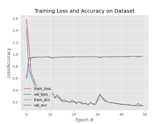Figure 10: Our malaria classifier model training/testing accuracy and loss plot shows that we’ve achieved high accuracy and low loss. The model isn’t exhibiting signs of over/underfitting. This deep learning medical imaging “malaria classifier” model was created with ResNet architecture using Keras.

Here we can see that our model was trained for a total of 50 epochs.

Each epoch tales approximately 65 seconds on a single Titan X GPU.

Overall, the entire training process took only 54 minutes (significantly faster than the 24-hour training process of NIH’s method). At the end of the 50th epoch we are obtaining:

• 96.50% accuracy on the training data

• 96.78% accuracy on the validation data

• 97% accuracy on the testing data

There are a number of benefits to using the ResNet-based model we trained here today for medical image analysis.

To start, our model is a complete end-to-end malaria classification system.

Unlike NIH’s approach which leverages a multiple step process of (1) feature extraction from multiple models and (2) classification, we instead can utilize only a single, compact model and obtain comparable results.

Speaking of compactness, our serialized model file is only 17.7MB. Quantizing the weights in the model themselves would allow us to obtain a model < 10MB (or even smaller, depending on the quantization method) with only slight, if any, decreases in accuracy.

Our approach is also faster in two manners.

First, it takes less time to train our model than NIH’s approach.

Our model took only 54 minutes to train while NIH’s model took ~24 hours.

Secondly, our model is faster in terms of both (1) forward-pass inference time and (2) significantly fewer parameters and memory/hardware requirements.

Consider the fact that NIH’s method requires pre-trained networks for feature extraction.

Each of these models accepts input images that have input image spatial dimensions in the range of 224×244, 227×227, and 299×299 pixels.

Our model requires only 64×64 input images and obtains near identical accuracy.

All that said, I have not performed a full-blown accuracy, sensitivity, and specificity test, but based on our results we can see that we are on the right track to creating an automatic malaria classifier that is not only more accurate but significantly smaller, requiring less processing power as well.

My hope is that you will use the knowledge in today’s tutorial on deep learning and medical imaging analysis and apply it to your own medical imaging problems.

Summary

In today’s blog post you learned how to apply deep learning to medical image analysis; specifically, malaria prediction.

Malaria is an infectious disease that often spreads through mosquitoes. Given the fast reproduction cycle of mosquitoes, malaria has become a true endemic in some areas of the world and an epidemic in others. In total, over 400,000 deaths per year can be attributed to malaria.

NIH has developed a mobile application, that when combined with a special microscope attachment lens on a smartphone, enables field clinicians to automatically predict malaria risk factors for a patient given a blood smear. NIH’s model combined six separate state-of-the-art deep learning models and took approximately 24 hours to train.

Overall, they obtained ~95.9% accuracy.

Using the model discussed in today’s tutorial, a smaller variant of ResNet whose model size is only 17.7MB, we were able to obtain 97% accuracy in only 54 minutes.

Furthermore, 75%+ of the code utilized in today’s tutorial came from my book, Deep Learning for Computer Vision with Python.

It took very little effort to take the code examples and techniques learned from the book and then apply it a custom medical image analysis problem.

During a disease outbreak, when time is of the essence, being able to leverage existing code and models can reduce engineer/training time, ensure the model is out in the field faster, and ultimately help doctors and clinicians better treat patients (and ideally save lives as well).

I hope you enjoyed today’s post on deep learning for medical image analysis!

To download the source code to today’s post, and be notified when future posts are published here on PyImageSearch, just enter your email address in the form below!

Downloads: