Marginal Effects for (mixed effects) regression models

ggeffects (CRAN, website) is a package that computes marginal effects at the mean (MEMs) or representative values (MERs) for many different models, including mixed effects or Bayesian models. One of the advantages of the package is its easy-to-use interface: No matter if you fit a simple or complex model, with interactions or splines, the function call is always the same. This also holds true for the returned output, which is always a data frame with the same, consistent column names.

The past package-update introduced some new features I wanted to describe here: a revised print()-method as well as a new opportunity to plot marginal effects at different levels of random effects in mixed models…

The new print()-method

The former print()-method simply showed the first predicted values, including confidence intervals. For numeric predictor variables with many values, you could, for instance, only see the first 10 of more than 100 predicted values. While it makes sense to shorten the (console-)output, there was no information about the predictions for the last or other „representative“ values of the term in question. Now, the print()-method automatically prints a selection of representative values, so you get a quick and clean impression of the range of predicted values for continuous variables:

library(ggeffects)
data(efc)
efc$c172code <- as.factor(efc$c172code)
fit <- lm(barthtot ~ c12hour * c172code + neg_c_7, data = efc)

ggpredict(fit, "c12hour")
#> 
#> # Predicted values of Total score BARTHEL INDEX 
#> # x = average number of hours of care per week 
#> 
#> x predicted std.error conf.low conf.high
#> 0 72.804 2.516 67.872 77.736
#> 20 68.060 2.097 63.951 72.170
#> 45 62.131 1.824 58.555 65.706
#> 65 57.387 1.886 53.691 61.083
#> 85 52.643 2.179 48.373 56.913
#> 105 47.900 2.626 42.752 53.047
#> 125 43.156 3.164 36.955 49.357
#> 170 32.482 4.531 23.602 41.363
#> 
#> Adjusted for:
#> * c172code = 1
#> * neg_c_7 = 11.83

If you print predicted values of a term, grouped by the levels of another term (which makes sense in the above example due to the present interaction), the print()-method automatically adjusts the range of printed values to keep the console-output short. In the following example, only 6 instead of 8 values per „block“ are shown:

ggpredict(fit, c("c12hour", "c172code"))
#> 
#> # Predicted values of Total score BARTHEL INDEX 
#> # x = average number of hours of care per week 
#> 
#> # c172code = 1
#> x predicted std.error conf.low conf.high
#> 0 72.804 2.516 67.872 77.736
#> 30 65.689 1.946 61.874 69.503
#> 55 59.759 1.823 56.186 63.331
#> 85 52.643 2.179 48.373 56.913
#> 115 45.528 2.887 39.870 51.186
#> 170 32.482 4.531 23.602 41.363
#> 
#> # c172code = 2
#> x predicted std.error conf.low conf.high
#> 0 76.853 1.419 74.073 79.633
#> 30 68.921 1.115 66.737 71.106
#> 55 62.311 1.122 60.112 64.510
#> 85 54.379 1.438 51.560 57.198
#> 115 46.447 1.934 42.656 50.238
#> 170 31.905 3.007 26.011 37.800
#> 
#> # c172code = 3
#> x predicted std.error conf.low conf.high
#> 0 73.862 2.502 68.958 78.766
#> 30 66.925 1.976 63.053 70.798
#> 55 61.145 2.155 56.920 65.369
#> 85 54.208 2.963 48.400 60.016
#> 115 47.271 4.057 39.320 55.222
#> 170 34.554 6.303 22.200 46.907
#> 
#> Adjusted for:
#> * neg_c_7 = 11.83

Marginal effects at specific levels of random effects

Marginal effects can also be calculated for each group level in mixed models. Simply add the name of the related random effects term to the terms-argument, and set type = "re". In the following example, we fit a linear mixed model and first simply plot the marginal effetcs, not conditioned on random effects.

library(sjlabelled)
library(lme4)
data(efc)
efc$e15relat <- as_label(efc$e15relat)
m <- lmer(neg_c_7 ~ c12hour + c160age + c161sex + (1 | e15relat), data = efc)
me <- ggpredict(m, terms = "c12hour")
plot(me)

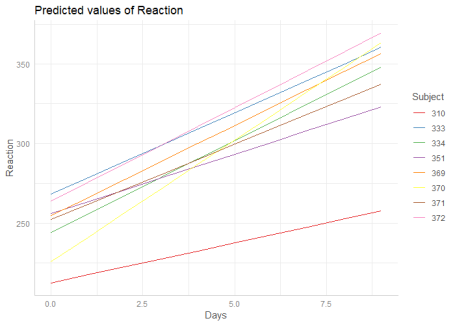
To compute marginal effects for each grouping level, add the related random term to the terms-argument. In this case, confidence intervals are not calculated, but marginal effects are conditioned on each group level of the random effects.

me <- ggpredict(m, terms = c("c12hour", "e15relat"), type = "re")
plot(me)

Marginal effects, conditioned on random effects, can also be calculated for specific levels only. Add the related values into brackets after the variable name in the terms-argument.

me <- ggpredict(m, terms = c("c12hour", "e15relat [child,cousin]"), type = "re")
plot(me)

If the group factor has too many levels, you can also take a random sample of all possible levels and plot the marginal effects for this subsample of group levels. To do this, use term = "groupfactor [sample=n]".

data("sleepstudy")
m <- lmer(Reaction ~ Days + (1 + Days | Subject), data = sleepstudy)
me <- ggpredict(m, terms = c("Days", "Subject [sample=8]"), type = "re")
plot(me)

Related