Instance segmentation with OpenCV

In this tutorial, you will learn how to perform instance segmentation with OpenCV, Python, and Deep Learning.

Back in September, I saw Microsoft release a really neat feature to their Office 365 platform — the ability to be on a video conference call, blur the background, and have your colleagues only see you (and not whatever is behind you).

The GIF at the top of this post demonstrates a similar feature that I have implemented for the purposes of today’s tutorial.

Whether you’re taking the call from a hotel room, working from a downright ugly office building, or simply don’t want to clean up around the home office, the conference call blurring feature can keep the meeting attendees focused on you (and not the mess in the background).

Such a feature would be especially helpful for people working from home and wanting to preserve the privacy of their family members.

Imagine your workstation being in clear view of your kitchen — you wouldn’t want your colleagues watching your kids eating dinner or doing their homework! Instead, just pop on the blurring feature and you’re all set.

In order to build such a feature, Microsoft leveraged computer vision, deep learning, and most notably, instance segmentation.

We covered Mask R-CNNs for instance segmentation in last week’s blog post — today we are going to take our Mask R-CNN implementation and use it to build a Microsoft Office 365-like video blurring feature.

To learn how to perform instance segmentation with OpenCV, just keep reading!

Instance segmentation with OpenCV

Today’s tutorial is inspired by both (1) Microsoft’s Office 365 video call blurring feature and (2) PyImageSearch reader Zubair Ahmed. Zubair implemented a similar blurring feature using Google’s DeepLab (you can find his implementation on his blog).

Since we covered instance segmentation in last week’s blog post, I thought it was the perfect time to demonstrate how we can mimic the call blurring feature using OpenCV.

In the first part of this tutorial, we’ll briefly cover instance segmentation. From there we’ll use instance segmentation and OpenCV to:

1. Detect and segment the user from the video stream

2. Blur the background

3. And then add the user back to the stream itself.

From there we’ll look at the results of our OpenCV instance segmentation algorithm, including some of the limitations and drawbacks.

What is instance segmentation?

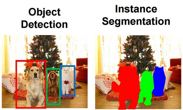
Figure 1: The difference between object detection and instance segmentation. For object detection (left), a box is drawn around the individual objects. In the case of instance segmentation (right), an attempt is made to determine which pixels belong to each object. (source)

Explaining instance segmentation is best done with a visual example — refer to Figure 1 above where we have an example of object detection on the left and instance segmentation on the right.

Looking at these two examples we can clearly see a difference between the two.

When performing object detection we are:

1. Computing the bounding box (x, y)-coordinates for each object

2. And then associating a class label with each bounding box as well.

The problem is that object detection tells us nothing regarding the shape of the object itself — all we have is a set of bounding box coordinates. Instance segmentation, on the other hand, computes a pixel-wise mask for each object in the image.

Even if the objects are of the same class label, such as the two dogs in the above image, our instance segmentation algorithm still reports a total of three unique objects: two dogs and one cat.

Using instance segmentation we now have a more granular understanding of the object in the image — we know specifically which (x, y)-coordinates the object exists in.

Furthermore, by using instance segmentation we can easily segment our foreground objects from the background.

We’ll be using a Mask R-CNN for instance segmentation in this post.

For a more detailed review of instance segmentation, including comparing and contrasting image classification, object detection, semantic segmentation, *and instance segmentation,* please refer to last week’s blog post.

Project structure

You can grab the source code and trained Mask R-CNN model from the “Downloads” section of today’s post.

Once you’ve extracted the archive and navigated into it, simply take advantage of the tree command to view the directory structure in your terminal:

$ tree –dirsfirst.├── mask-rcnn-coco│ ├── frozen_inference_graph.pb│ ├── mask_rcnn_inception_v2_coco_2018_01_28.pbtxt│ └── object_detection_classes_coco.txt└── instance_segmentation.py 1 directory, 4 files

.

│ ├── frozen_inference_graph.pb

│ └── object_detection_classes_coco.txt

 

Our project includes one directory (consisting of three files) and one Python script:

mask-rcnn-coco/ : The Mask R-CNN model directory contains three files:

frozen_inference_graph.pb : The Mask R-CNN model weights. The weights are pre-trained on the COCO dataset.

mask_rcnn_inception_v2_coco_2018_01_28.pbtxt : The Mask R-CNN model configuration. If you’d like to build + train your own model on your own annotated data, refer to Deep Learning for Computer Vision with Python.

object_detection_classes_coco.txt : All 90 classes are listed in this text file, one per line. Open it in a text editor to see what objects our model can recognize.

Implementing instance segmentation with OpenCV

Let’s get started implementing instance segmentation with OpenCV.

Open up the instance_segmentation.py file and insert the following code:

# import the necessary packagesfrom imutils.video import VideoStreamimport numpy as npimport argparseimport imutilsimport timeimport cv2import os

from imutils.video import VideoStream

import argparse

import time

import os

We’ll start off the script by importing our necessary packages. You need the following installed in your environment (virtual environments are highly recommended):

• OpenCV 3.4.2+ — If you don’t have OpenCV installed, head over to my installation tutorials page. The fastest method for installing on most systems is via pip which will install OpenCV 3.4.3 at the time of this writing.

imutils — This is my personal package of computer vision convenience functions. You may install imutils via: pip install –upgrade imutils .

Again, I highly recommend that you place this software in an isolated virtual environment as you may need to accommodate for different versions for other projects.

Let’s parse our command line arguments:

# construct the argument parse and parse the argumentsap = argparse.ArgumentParser()ap.add_argument(“-m”, “–mask-rcnn”, required=True, help=”base path to mask-rcnn directory”)ap.add_argument(“-c”, “–confidence”, type=float, default=0.5, help=”minimum probability to filter weak detections”)ap.add_argument(“-t”, “–threshold”, type=float, default=0.3, help=”minimum threshold for pixel-wise mask segmentation”)ap.add_argument(“-k”, “–kernel”, type=int, default=41, help=”size of gaussian blur kernel”)args = vars(ap.parse_args())

ap = argparse.ArgumentParser()

help=”base path to mask-rcnn directory”)

help=”minimum probability to filter weak detections”)

help=”minimum threshold for pixel-wise mask segmentation”)

help=”size of gaussian blur kernel”)

Descriptions of each command line argument can be found below:

–mask-rcnn : The base path to the Mask R-CNN directory. We reviewed the three files in this directory in the “Project structure” section above.

–confidence : The minimum probability to filter out weak detections. I’ve set this value to a default of 0.5 , but you can easily pass different values via the command line.

–threshold : Our minimum threshold for the pixel-wise mask segmentation. The default is set to 0.3 .

–kernel : The size of the Gaussian blur kernel. I found that a 41 x 41 kernel looks pretty good, so a default of 41 is set.

For a review on how command line arguments work, be sure to read this guide.

Let’s load our labels and our OpenCV instance segmentation model:

222324252627282930313233343536

# load the COCO class labels our Mask R-CNN was trained onlabelsPath = os.path.sep.join([args[“mask_rcnn”], “object_detection_classes_coco.txt”])LABELS = open(labelsPath).read().strip().split(“\n”) # derive the paths to the Mask R-CNN weights and model configurationweightsPath = os.path.sep.join([args[“mask_rcnn”], “frozen_inference_graph.pb”])configPath = os.path.sep.join([args[“mask_rcnn”], “mask_rcnn_inception_v2_coco_2018_01_28.pbtxt”]) # load our Mask R-CNN trained on the COCO dataset (90 classes)# from diskprint(“[INFO] loading Mask R-CNN from disk…“)net = cv2.dnn.readNetFromTensorflow(weightsPath, configPath)

23

25

27

29

31

33

35

labelsPath = os.path.sep.join([args[“mask_rcnn”],

LABELS = open(labelsPath).read().strip().split(“\n”)

derive the paths to the Mask R-CNN weights and model configuration

“frozen_inference_graph.pb”])

“mask_rcnn_inception_v2_coco_2018_01_28.pbtxt”])

load our Mask R-CNN trained on the COCO dataset (90 classes)

print(“[INFO] loading Mask R-CNN from disk…”)

Our labels file needs to be located in the mask-rcnn-coco/ directory — the directory specified via command line argument. Lines 23 and 24 build the labelsPath and then Line 25 reads the LABELS into a list.

The same goes for our weightsPath and configPath which are built on Lines 28-31.

Using these two paths, we take advantage of the dnn module to initialize the neural net (Line 36). This call loads the Mask R-CNN into memory before we start processing frames (we only need to load it once).

Let’s construct our blur kernel and start our webcam video stream:

# construct the kernel for the Gaussian blur and initialize whether# or not we are in “privacy mode”K = (args[“kernel”], args[“kernel”])privacy = False # initialize the video stream, then allow the camera sensor to warm upprint(“[INFO] starting video stream…“)vs = VideoStream(src=0).start()time.sleep(2.0)

or not we are in “privacy mode”

privacy = False

initialize the video stream, then allow the camera sensor to warm up

vs = VideoStream(src=0).start()

The blur kernel tuple is defined on Line 40.

Our project has two modes: “normal mode” and “privacy mode”. Thus, a privacy boolean is used for the mode logic. It is initialized to False on Line 41.

Our webcam video stream is started on Line 45 where we pause for two seconds to allow the sensor to warm up (Line 46).

Now that all of our variables and objects are initialized, let’s start processing frames from the webcam:

48495051525354555657585960616263646566

# loop over frames from the video file streamwhile True: # grab the frame from the threaded video stream frame = vs.read()  # resize the frame to have a width of 600 pixels (while # maintaining the aspect ratio), and then grab the image # dimensions frame = imutils.resize(frame, width=600) (H, W) = frame.shape[:2]  # construct a blob from the input image and then perform a # forward pass of the Mask R-CNN, giving us (1) the bounding # box coordinates of the objects in the image along with (2) # the pixel-wise segmentation for each specific object blob = cv2.dnn.blobFromImage(frame, swapRB=True, crop=False) net.setInput(blob) (boxes, masks) = net.forward([“detection_out_final”, “detection_masks”])

49

51

53

55

57

59

61

63

65

while True:

frame = vs.read()

# resize the frame to have a width of 600 pixels (while

# dimensions

(H, W) = frame.shape[:2]

# construct a blob from the input image and then perform a

# box coordinates of the objects in the image along with (2)

blob = cv2.dnn.blobFromImage(frame, swapRB=True, crop=False)

(boxes, masks) = net.forward([“detection_out_final”,

Our frame processing loop begins on Line 49.

At each iteration, we’ll grab a frame (Line 51) and resize it to a known width, maintaining aspect ratio (Line 56).

For scaling purposes later, we go ahead and extract the dimensions of the frame (Line 57).

Then, we construct a blob and complete a forward pass through the network (Lines 63-66). You can read more about how this process works in this previous blog post.

The result is both boxes and masks . We’ll be taking advantage of the masks , but we also need to use the data contained in boxes .

Let’s sort the indexes and initialize variables:

# sort the indexes of the bounding boxes in by their corresponding # prediction probability (in descending order) idxs = np.argsort(boxes[0, 0, :, 2])[::-1]  # initialize the mask, ROI, and coordinates of the person for the # current frame mask = None roi = None coords = None

# prediction probability (in descending order)

 

# current frame

roi = None

Line 70sorts the indexes of the bounding boxes by their corresponding prediction probability. We’ll be making the assumption that the person with the largest corresponding detection probability is our user.

We then initialize the mask , roi , and bounding box coords (Lines 74-76).

Let’s loop over the indexes and filter the results:

78798081828384858687888990919293949596979899100

# loop over the indexes for i in idxs: # extract the class ID of the detection along with the # confidence (i.e., probability) associated with the # prediction classID = int(boxes[0, 0, i, 1]) confidence = boxes[0, 0, i, 2]  # if the detection is not the ‘person’ class, ignore it if LABELS[classID] != “person”: continue  # filter out weak predictions by ensuring the detected # probability is greater than the minimum probability if confidence > args[“confidence”]: # scale the bounding box coordinates back relative to the # size of the image and then compute the width and the # height of the bounding box box = boxes[0, 0, i, 3:7] * np.array([W, H, W, H]) (startX, startY, endX, endY) = box.astype(“int”) coords = (startX, startY, endX, endY) boxW = endX - startX boxH = endY - startY

79

81

83

85

87

89

91

93

95

97

99

for i in idxs:

# confidence (i.e., probability) associated with the

classID = int(boxes[0, 0, i, 1])

 

if LABELS[classID] != “person”:

 

# probability is greater than the minimum probability

# scale the bounding box coordinates back relative to the

# height of the bounding box

(startX, startY, endX, endY) = box.astype(“int”)

boxW = endX - startX

We begin looping over the idxs on Line 79.

We then extract the classID and confidence using boxes and the current index (Lines 83 and 84).

Subsequently, we’ll perform our first filter — we only care about the “person” class. If any other object class is encountered, we’ll continue to the next index (Lines 87 and 88).

Our next filter ensures the confidence of the prediction exceeds the threshold set via command line arguments (Line 92).

If we pass that test, then we’ll scale the bounding box coordinates back to the relative dimensions of the image (Lines 96). We then extract the coords and object width/height (Lines 97-100).

Let’s compute our mask and extract the ROI:

102103104105106107108109110111112113114115116

# extract the pixel-wise segmentation for the object, # resize the mask such that it’s the same dimensions of # the bounding box, and then finally threshold to create # a binary mask mask = masks[i, classID] mask = cv2.resize(mask, (boxW, boxH), interpolation=cv2.INTER_NEAREST) mask = (mask > args[“threshold”])  # extract the ROI and break from the loop (since we make # the assumption there is only one person in the frame # who is also the person with the highest prediction # confidence) roi = frame[startY:endY, startX:endX][mask] break

103

105

107

109

111

113

115

# resize the mask such that it’s the same dimensions of

# a binary mask

mask = cv2.resize(mask, (boxW, boxH),

mask = (mask > args[“threshold”])

# extract the ROI and break from the loop (since we make

# who is also the person with the highest prediction

roi = frame[startY:endY, startX:endX][mask]

Lines 106-109 extract the mask , resize it, and apply the threshold to create the binary mask itself. An example mask is shown in Figure 2:

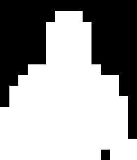
Figure 2: The binary mask computed via instance segmentation of me in front of my webcam using OpenCV and instance segmentation. Computing the mask is part of the privacy filter pipeline.

In Figure 2 above all white pixels are assumed to be a person (i.e., the foreground) while all black pixels are the background.

With the mask , we’ll also compute the roi (Line 115) via NumPy array slicing.

We then break from the loop on Line 116 (since we have found the “person” with the largest probability).

Let’s initialize our output frame and compute our blur if we are in “privacy mode”:

118119120121122123124125126127128129

# initialize our output frame output = frame.copy()  # if the mask is not None and we are in privacy mode, then we # know we can apply the mask and ROI to the output image if mask is not None and privacy: # blur the output frame output = cv2.GaussianBlur(output, K, 0)  # add the ROI to the output frame for only the masked region (startX, startY, endX, endY) = coords output[startY:endY, startX:endX][mask] = roi

119

121

123

125

127

129

output = frame.copy()

# if the mask is not None and we are in privacy mode, then we

if mask is not None and privacy:

output = cv2.GaussianBlur(output, K, 0)

# add the ROI to the output frame for only the masked region

output[startY:endY, startX:endX][mask] = roi

Our output frame is simply a copy of the original frame (Line 119).

If we both:

Have a mask that is not empty And we are in ” privacy mode”…

…then we’ll blur the background (using our kernel) and apply the mask to the output frame (Lines 123-129).

Now let’s display the output image and handle keypresses:

131132133134135136137138139140141142143144145

# show the output frame cv2.imshow(“Video Call”, output) key = cv2.waitKey(1) & 0xFF  # if the p key was pressed, toggle privacy mode if key == ord(“p”): privacy = not privacy  # if the q key was pressed, break from the loop elif key == ord(“q”): break # do a bit of cleanupcv2.destroyAllWindows()vs.stop()

132

134

136

138

140

142

144

cv2.imshow(“Video Call”, output)

 

if key == ord(“p”):

 

elif key == ord(“q”):

 

cv2.destroyAllWindows()

Our output frame is displayed via Line 132.

Keypresses are captured (Line 133). Two keys cause different behaviors (Lines 136-141):

“p” : When this key is pressed, “ privacy mode” is toggled either on or off.

“q” : If this key is pressed, we’ll break out of the loop and “quit” the script.

Whenever we do quit, Lines 144and 145 close the open window and stop the video stream.

Instance segmentation results

Now that we’ve implemented our OpenCV instance segmentation algorithm, let’s see it in action!

Be sure to use the “Downloads� section of this blog post to download the code and Mask R-CNN model.

From there, open up a terminal and execute the following command:

$ python instance_segmentation.py –mask-rcnn mask-rcnn-coco –kernel 41[INFO] loading Mask R-CNN from disk…[INFO] starting video stream…

[INFO] loading Mask R-CNN from disk…

Figure 3: My demonstration of a “privacy filter” for web chatting. I’ve used OpenCV and Python to perform instance segmentation to find the prominent person (me), and then applied blurring to the background.

Here you can see a short GIF of me demoing our instance segmentation pipeline.

In this image, I am meant to be the “conference call attendee�. Trisha, my wife, is working in the background.

By enabling “privacy mode� I can:

1. Use OpenCV instance segmentation to find the person detection with the largest corresponding probability (most likely that will be the person closest to the camera).

2. Blur the background of the video stream.

3. Overlay the segmented, non-blurry person back onto the video stream.

I have included a video demo, including my commentary, below:

You’ll immediately notice that we are not obtaining true real-time performance though — we’re only processing a few frames per second. Why is this?

How come our OpenCV instance segmentation pipeline isn’t faster?

To answer those questions, be sure to refer to the section below.

Limitations, drawbacks, and potential improvements

The first limitation is the most obvious one — our OpenCV instance segmentation implementation is too slow to run in real-time.

On my Intel Xeon W we’re only processing a few frames per second.

In order to obtain true real-time instance segmentation performance, we would need to leverage our GPU.

But therein lies the problem:

OpenCV’s GPU support for its dnn module is fairly limited.

Currently, it mainly supports Intel GPUs.

NVIDIA CUDA GPU support is in development, but is currently not available.

Once OpenCV officially supports NVIDIA GPUs for the dnn module we’ll be more easily able to build real-time (and even super real-time) deep learning applications.

But for now, this OpenCV instance segmentation tutorial serves as an educational demo of:

1. What’s currently possible

2. And what will be possible in a few months

Another improvement we can make is related to the overlaying of the segmented person back on the blurred background.

When you compare our implementation to Microsoft’s Office 365 video blurring feature, you’ll see that Microsoft’s is much more “smooth�.

We can mimic this feature by utilizing a bit of alpha blending.

A simple yet effective update to our instance segmentation pipeline would be to potentially:

1. Use morphological operations to increase the size of our mask

2. Apply a small amount of Gaussian blurring to the mask itself, helping smooth the mask

3. Scale the mask values to the range [0, 1]

4. Create an alpha layer using the scaled mask

5. Overlay the smoothed mask + person ROI on the blurred background

Alternatively, you could compute the contours of the mask itself and then apply contour approximation to help create a “more smoothed” mask.

Please note that I have not tried this algorithm — it’s just something I thought of off the top of my head that I thought could give visually pleasing results.

If you wish to implement this instance segmentation update I would suggest reading this post where I discuss alpha blending in more detail.

Summary

In today’s blog post you learned how to perform instance segmentation using OpenCV, Deep Learning, and Python.

Instance segmentation is the process of:

1. Detecting each object in an image

2. Computing a pixel-wise mask for each object

Even if objects are of the same class, an instance segmentation should return a unique mask for each object.

In order to apply instance segmentation with OpenCV, we used our Mask R-CNN implementation from last week.

We then used our Mask R-CNN model to build a “video conference call blurring feature�, similar to the feature Microsoft released for Office 365 back in the summer.

Our instance segmentation results were similar to Microsoft’s feature; however, we could not obtain true real-time performance since OpenCV’s GPU support for the dnn module is currently quite limited.

Therefore, today’s tutorial serves as a demo, highlighting what is currently possible and what will be possible when OpenCV’s GPU support increases.

I hope you enjoyed today’s tutorial!

To download the source code to this post, and be notified when future tutorials are published here on PyImageSearch, just enter your email address in the form below!

Downloads: