By George Seif, AI / Machine Learning Engineer
Statistics can be a powerful tool when performing the art of Data Science (DS). From a high-level view, statistics is the use of mathematics to perform technical analysis of data. A basic visualisation such as a bar chart might give you some high-level information, but with statistics we get to operate on the data in a much more information-driven and targeted way. The math involved helps us form concrete conclusions about our data rather than just guesstimating.
Using statistics, we can gain deeper and more fine grained insights into how exactly our data is structured and based on that structure how we can optimally apply other data science techniques to get even more information. Today, we’re going to look at 5 basic statistics concepts that data scientists need to know and how they can be applied most effectively!
Statistical Features
Statistical features is probably the most used statistics concept in data science. It’s often the first stats technique you would apply when exploring a dataset and includes things like bias, variance, mean, median, percentiles, and many others. It’s all fairly easy to understand and implement in code! Check out the graphic below for an illustration.
The line in the middle is the median value of the data. Median is used over the mean since it is more robust to outlier values. The first quartile is essentially the 25th percentile; i.e 25% of the points in the data fall below that value. The third quartile is the 75th percentile; i.e 75% of the points in the data fall below that value. The min and max values represent the upper and lower ends of our data range.
A box plot perfectly illustrates what we can do with basic statistical features:
When the box plot is shortit implies that much of your data points are similar, since there are many values in a small range When the box plot is tall it implies that much of your data points are quite different, since the values are spread over a wide range If the median value is closer to the bottom then we know that most of the data has lower values. If the median value is closer to the top then we know that most of the data has higher values. Basically, if the median line is not in the middle of the box then it is an indication of skewed data. Are the whiskers very long? That means your data has a high standard deviationand variancei.e the values are spread out and highly varying. If you have long whiskers on one side of the box but not the other, then your data may be highly varying only in one direction.
All of that information from a few simple statistical features that are easy to calculate! Try these out whenever you need a quick yet informative view of your data.
Probability Distributions
We can define probability as the percent chance that some event will occur. In data science this is commonly quantified in the range of 0 to 1 where 0 means we are certain this will not occur and 1 means we are certain it will occur. A probability distribution is then a function which represents the probabilities of all possible values in the experiment. Check out the graphic below for an illustration.
 Common Probability Distributions. Uniform (left), Normal (middle), Poisson (right)
AUniform Distribution is the most basic of the 3 we show here. It has a single value which only occurs in a certain range while anything outside that range is just 0. It’s very much an “on or off” distribution. We can also think of it as an indication of a categorical variable with 2 categories: 0 or the value. Your categorical variable might have multiple values other than 0 but we can still visualize it in the same was as a piecewise function of multiple uniform distributions. A Normal Distribution, commonly referred to as a GaussianDistribution,is specifically defined by its mean and standard deviation. The mean value shifts the distribution spatially and the standard deviation controls the spread. The import distinction from other distributions (e.g poisson) is that the standard deviation is the same in all directions. Thus with a Gaussian distribution we know the average value of our dataset as well as the spread of the data i.e is it spread over a wide range or is it highly concentrated around a few values. A Poisson Distributionis similar to the Normal but with an added factor of skewness. With a low value for the skewness a poisson distribution will have relatively uniform spread in all directions just like the Normal. But when the skewness value is high in magnitude then the spread of our data will be different in different directions; in one direction it will be very spread and in the other it will be highly concentrated.
There are many more distributions that you can dive deep into but those 3 already give us a lot of value. We can quickly see and interpret our categorical variables with a Uniform Distribution. If we see a Gaussian Distribution we know that there are many algorithms that by default will perform well specifically with Gaussian so we should go for those. And with Poisson we’ll see that we have to take special care and choose an algorithm that is robust to the variations in the spatial spread.
Dimensionality Reduction
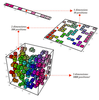
The term Dimensionality Reduction is quite intuitive to understand. We have a dataset and we would like to reduce the number of dimensions it has. In data science this is the number of feature variables. Check out the graphic below for an illustration.
 Dimensionality Reduction
The cube represents our dataset and it has 3 dimensions with a total of 1000 points. Now with today’s computing 1000 points is easy to process, but at a larger scale we would run into problems. However, just by looking at our data from a 2-Dimensional point of view, such as from one side of the cube, we can see that it’s quite easy to divide all of the colours from that angle. With dimensionality reduction we would then project the 3D data onto a 2D plane. This effectively reduces the number of points we need to compute on to 100, a big computational saving!
Another way we can do dimensionality reduction is through feature pruning. With feature pruning we basically want to remove any features we see will be unimportant to our analysis. For example, after exploring a dataset we may find that out of the 10 features, 7 of them have a high correlation with the output but the other 3 have very low correlation. Then those 3 low correlation features probably aren’t worth the compute and we might just be able to remove them from our analysis without hurting the output.
The most common stats technique used for dimensionality reduction is PCA which essentially creates vector representations of features showing how important they are to the output i.e their correlation. PCA can be used to do both of the dimensionality reduction styles discussed above. Read more about it in this tutorial.
Over and Under Sampling
Over and Under Sampling are techniques used for classification problems. Sometimes, our classification dataset might be too heavily tipped to one side. For example, we have 2000 examples for class 1, but only 200 for class 2. That’ll throw off a lot of the Machine Learning techniques we try and use to model the data and make predictions! Our Over and Under Sampling can combat that. Check out the graphic below for an illustration.
 Under and and Over Sampling
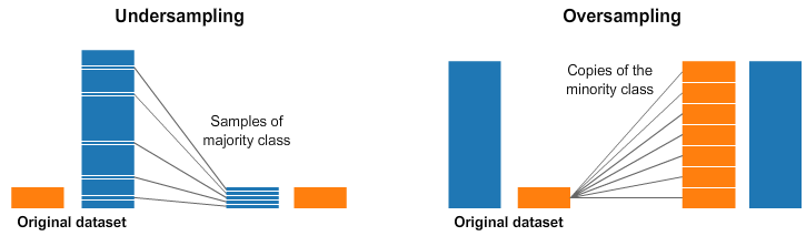
In both the left and right side of the image above, our blue class has far more samples than the orange class. In this case, we have 2 pre-processing options which can help in the training of our Machine Learning models.
Undersampling means we will select only some of the data from the majority class, only using as many examples as the minority class has. This selection should be done to maintain the probability distribution of the class. That was easy! We just evened out our dataset by just taking less samples!Oversampling means that we will create copies of our minority class in order to have the same number of examples as the majority class has. The copies will be made such that the distribution of the minority class is maintained. We just evened out our dataset without getting any more data!
Bayesian Statistics
Fully understanding why we use Bayesian Statistics requires us to first understand where Frequency Statistics fails. Frequency Statistics is the type of stats that most people think about when they hear the word “probability”. It involves applying math to analyze the probability of some event occurring, where specifically the only data we compute on is prior data.
Let’s look at an example. Suppose I gave you a die and asked you what were the chances of you rolling a 6. Well most people would just say that it’s 1 in 6. Indeed if we were to do a frequency analysis we would look at some data where someone rolled a die 10,000 times and compute the frequency of each number rolled; it would roughly come out to 1 in 6!
But what if someone were to tell you that the specific die that was given to youwas loaded to always land on 6? Since frequency analysis only takes into account prior data, that evidence that was given to you about the die being loaded is notbeing**taken into account.
Bayesian Statistics does take into account this evidence. We can illustrate this by taking a look at Baye’s theorem:
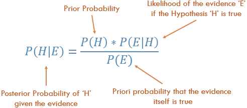 Baye’s Theoram
| The probability P(H) in our equation is basically our frequency analysis; given our prior data what is the probability of our event occurring. The *P(E | H) in our equation is called the likelihood and is essentially the probability that our evidence is correct, given the information from our frequency analysis. For example, if you wanted to roll the die 10,000 times, and the first 1000 rolls you got all 6 you’d start to get pretty confident that that die is loaded! The P(E) *is the probability that the actual evidence is true. If I told you the die is loaded, can you trust me and say it’s actually loaded or do you think it’s a trick?! |
If our frequency analysis is very good then it’ll have some weight in saying that yes our guess of 6 is true. At the same time we take into account our evidence of the loaded die, if it’s true or not based on both its own prior and the frequency analysis. As you can see from the layout of the equation Bayesian statistics takes everything into account. Use it whenever you feel that your prior data will not be a good representation of your future data and results.
A Data Science book
Want to learn more about data science? This book is seriously the best I’ve seen on the subject offering practical and easy to understand lessons.
Like to learn?
Follow me on twitter where I post all about the latest and greatest AI, Technology, and Science!
Bio: George Seif is a Certified Nerd and AI / Machine Learning Engineer.
Original. Reposted with permission.
Related: