Time Series and MCHT

Introduction Over the past few weeks I’ve published articles about my new package, MCHT, starting with an introduction, a further technical discussion, demonstrating maximized Monte Carlo (MMC) hypothesis testing, bootstrap hypothesis testing, and last week I showed how to handle multi-sample and multivariate data. This is the final article where I explain the capabilities of the package. I show how MCHT can handle time series data.

I should mention that I’m not focused on the merits of the procedures I use as examples in these posts, and that’s going to be the case here. It’s possible (perhaps even likely) that there’s a better way to decide between the hypotheses than what I show here. In these articles, I’m more interested in showing what can be done rather than what should be done. In particular, I like simple examples that many can understand, even if they may not be the best tool for the task at hand.

So far I don’t think this has been a serious issue; that is, I don’t think the procedures I’ve shown so far could be considered controversial (I think the most controversial would be the permutation test example). But the example I want to use here could be argued with; I personally would not use it. That said, I’m still willing to demonstrate it because it doesn’t take much to understand what’s going on and it does demonstrate how time series data can be handled.

Context

Suppose we want to perform a test for the location of the mean, and thus decide between the hypotheses

$H_0: \mu = \mu_0$ $H_0: \mu = \mu_0$

$H_A: \mu \neq \mu_0$ $H_A: \mu \neq \mu_0$

There is the usual $t$ $t$ -statistic, which is $\frac{\bar{X} - \mu_0}{\frac{S}{\sqrt{n}}}$ $\frac{\bar{X} - \mu_0}{\frac{S}{\sqrt{n}}}$ , and as mentioned before the statistic assumes that the data came from a Normal distribution. That’s not all the test assumes, though. It also assumes that the data is independent and identically distributed.

In cross-sectional contexts this is fine, but it’s not okay when the data could depend on time and thus is not independent and identically distributed. Suppose instead that our data was generated according to a first-order autoregressive process (AR(1)), described below:

$X_t = \mu + \epsilon_t$ $X_t = \mu + \epsilon_t$

$\epsilon_t = \rho \epsilon_{t - 1} + \sigma w_t$ $\epsilon_t = \rho \epsilon_{t - 1} + \sigma w_t$

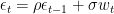
In this context, assume $w_t \sim N(0, 1)$ $w_t \sim N(0, 1)$ and is independent and identically distribution. It’s no longer given that the conventional $t$ $t$ -test will work as marketed since the data is no longer independent or identically distributed. Additionally, we have two nuisance parameters, $\rho$ $\rho$ and $\sigma$ $\sigma$ , that need to be accounted for.

Monte Carlo Testing with Time Series

We will view $\rho$ $\rho$ and $\sigma$ $\sigma$ as nuisance parameters and use MMC testing to handle them. That leaves the question of how to simulate an AR(1) process. With MCHT, if you can simulate a process, you can test with it.

The time series model above has a stationary solution when $|\rho| < 1$ $|\rho| < 1$ and when $t$ $t$ ranges between $-\infty$ $-\infty$ and $\infty$ $\infty$ . It’s not possible to simulate a series of infinite length but one can get close by simulating a series that is very long. In particular, one can simulate, say, 500 terms of the series starting at a fixed number, then the actual number of terms of the series wanted, then throw away the first 500 terms. This is known as burn-in and it’s very common practice in time series simulation.

Fortunately MCHTest() allows for burn-in. Suppose that the sample size of the actual dataset is $n$ $n$ and we’ve decided that we want a burn-in period of $B$ $B$ . Then we can do the following:

Generate $n + B$ $n + B$ random numbers to represent $w_t$ $w_t$ (except possibly for the scaling factor, as we’re treating that as a nuisance parameter). Apply the recursive formula described above to the $w_t$ $w_t$ series after scaling the series by $\sigma$ $\sigma$ and using a chosen $\rho$ $\rho$ , and add $\mu$ $\mu$ to it. Keep only the last $n$ $n$ terms of the series; throw away the rest. This is your simulated dataset.

After having obtained the simulated dataset, proceed with the Monte Carlo test as usual.

With MMC, the unscaled series $w_t$ $w_t$ is fixed after we generate it and we use optimization to adversarially choose $\rho$ $\rho$ and $\sigma$ $\sigma$ so that we maximize the $p$ $p$ -value of the test.

When using MCHTest(), the rand_gen function does not need to produce a dataset of the same length as the original dataset; this allows for burning it. However, if you’re going to do this, then the stat_gen function needs to know what the sample size of the dataset is, but all you need to do is give the stat_gen function the parameter n; this will be given the sample size of the original dataset. And of course the test_stat function won’t care whether the data came from a time series or not.

Putting this all together, we create the following test.

Conclusion

I have now covered what I consider the essential technical functionality of MCHT. All of the functionality I described in these posts is functionality that I want this package to have. Thus I personally am quite happy this package exists, which is good; I’m the package’s primary audience, after all. All I can hope is that others find the package useful too.

I wrote this article more than a month before it was published, so perhaps I have made an update that isn’t being accounted for here, but as of this version (0.1.0), I’d call the package in a beta stage of stability; it’s usable, but features could be added or removed and there could be unknown bugs.

The following is a list of possible areas of expansion. This list exists mostly because I think it needs to exist; it gives me something to aim for before making a 1.0 release. That said, they could be useful features.

A function for making diagnostic-type plots for tests, such as a function creating a plot for the rejection probability function (RPF) as described in [1].A function that accepts a MCHTest-class object and returns a function that, rather than returning a htest-class object, returns a function that will give the test statistic, simulated test statistics, and a $p$ $p$ -value, in a list; could be useful for diagnostic work.Real-world datasets that can be used for examples.Functions with a simpler interface than MCHTest, perhaps with more restrictions on inputs.*Pre-made MCHTest objects perhaps implementing common Monte Carlo or Bootstrap tests.

I also welcome community requests and collaboration. If you want a feature, consider issuing a pull request on GitHub.

Do you want more documentation? More examples? More background? Let me know! I’d be willing to write more on this subject. Perhaps if I amass enough content I could write a book documenting MCHT and Monte Carlo/bootstrap testing.

These blog posts together extend beyond 10,000 words, so I’m thinking I have enough material to submit an article to, say, J. Stat. Soft. or the R Journal and thus get my first publication where I’m the sole author. But this is something I’m still considering; I’m an insecure person at heart.

Next week I will still be using this package in a blog post, but I won’t be writing about how to use it anymore; instead, I’ll be using it to revisit a proposition I made many months ago. (It was because of that article I created this package.) Stay tuned, and thanks for reading!

References

R. Davidson and J. G. MacKinnon, The size distortion of bootstrap test, Econometric Theory, vol. 15 (1999) pp. 361-376

Packt Publishing published a book for me entitled Hands-On Data Analysis with NumPy and Pandas, a book based on my video course Unpacking NumPy and Pandas. This book covers the basics of setting up a Python environment for data analysis with Anaconda, using Jupyter notebooks, and using NumPy and pandas. If you are starting out using Python for data analysis or know someone who is, please consider buying my book or at least spreading the word about it. You can buy the book directly or purchase a subscription to Mapt and read it there.

If you like my blog and would like to support it, spread the word (if not get a copy yourself)!

Related