Building a neighbour matrix with python

At some point, I ended up with a model like this one:

Y~=W⋅Y\tilde{Y} = W \cdot Y Y~=W⋅Y

where W is a matrix that can be defined as (for example):

wij=1w_{ij} = 1 wij=1

if j is within the K nearest neighbours of i, 0 otherwise.

Here is the receipe I have used to create the W matrix using numpy, scipy and matplotlib for visualization.

If you are already familiar with scipy cKDTree and sparse matrix, you can directly go to the last section.

Sample data

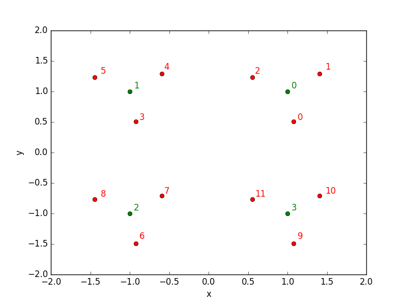
I have created a dummy dataset for the purpose of the demonstration, with sizes N=12 train samples and M=3 test samples:

import numpy as np
XY_train = np.array([[1.07712572, 0.50598419], [1.40709049, 1.29030559], [0.55806126, 1.23385926], [-0.92287428, 0.50598419], [-0.59290951, 1.29030559], [-1.44193874, 1.23385926], [-0.92287428, -1.49401581], [-0.59290951, -0.70969441], [-1.44193874, -0.76614074], [1.07712572, -1.49401581], [1.40709049, -0.70969441], [0.55806126, -0.76614074]])
XY_test = np.array([[1, 1], [-1, 1], [-1, -1], [1, -1]])

Let’s have a look at those points repartition: red points are the train data while the green points belon to the test data.

Find neighbours

Finding neighbours with the modern tools is quite straightforward. I choose here to use scipy because I will use other tools from this package later on in this post, but sklearn or other packages can also do the job. With scipy, first create a cKDTree with the train dataset:

from scipy.spatial import cKDTree
tree = cKDTree(XY_train)

tree that can be queried in a second time:

K = 3
result = tree.query(XY_test, k=K)

Here we asked for the three nearest neighbours in the train sample of the elements in the test sample. By default, tree.query returns both the neighbours indices and the distances involved. We’ll keep both of them.

distances, indices = result

Let’s concentrate on the indices array.

array([[0, 1, 2], [3, 4, 5], [6, 7, 8], [9, 10, 11]])

It is a numpy array with M (number of test samples) rows and K (number of neighbours) columns. How to transform this to the matrix we are looking for, that with our example should look like:

It can be interesting to see the selected neighbours on a plot:

import matplotlib.pyplot as plt
n = 0 # first element in the test dataset
xy_test = XY_test[n]
index = indices[n]
neighbours = XY_train[index]
plt.clf()
plt.scatter(xy_test[0], xy_test[1], color="red")
plt.scatter(neighbours[:,0], neighbours[:,1], color="blue")
plt.xlabel("x")
plt.ylabel("y")
plt.xlim(-2, 2)
plt.ylim(-2, 2)
plt.show()

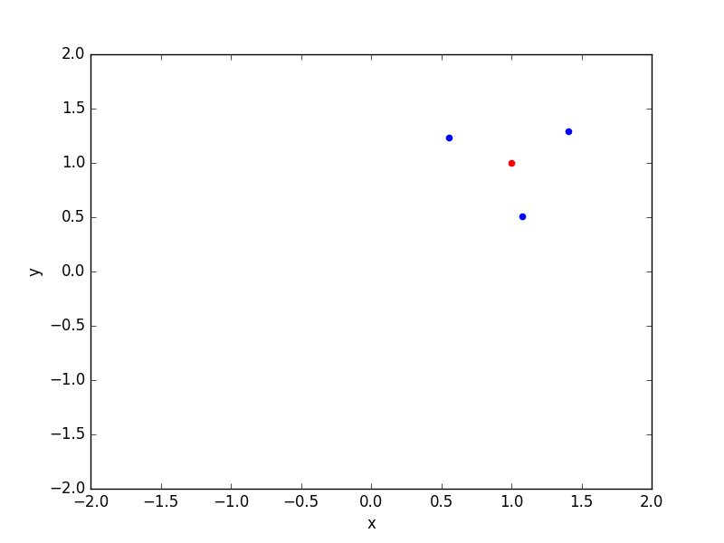
Ok so neighbours finding seems to work as expected! Let’s know see how to convert the indices array into a full usable matrix, that for our purpose should look like:

1 1 0 0 0 0 0 0 0 0 0
0 0 1 1 1 0 0 0 0 0 0
0 0 0 0 0 1 1 1 0 0 0
0 0 0 0 0 0 0 0 1 1 1

because the neighbours of test observation 0 (first row) are the train observations 0, 1 and 2, the neighbours of the test observation 1 (second row) are the train observations 3, 4 and 5, and so on.

Matrix creation

At first, we would like to use numpy indexing to create our matrix like this

import numpy as np
a = np.array([1, 2, 3, 4, 5, 6])
i = [0, 0, 1, 1, 2, 2]
a[i]
# array([1, 1, 2, 2, 3, 3])

but you’ll realize it doesn’t work on more than one dimension arrays.

The solution I choose is to use scipy sparse matrices, that can be created from a list of indices. For example, creating the diagonal matrix of size N=4 with sparse matrix can be written as:

from scipy import sparse
i_index = [0, 1, 2, 3]
j_index = [0, 1, 2, 3]
values = [1, 1, 1, 1]
matrix = sparse.coo_matrix((values, (i_index, j_index)), shape=(4, 4))
print(matrix)
# (0, 0)1
# (1, 1)1
# (2, 2)1
# (3, 3)1

So scipy takes the first elements of i_index and j_index arrays, i and j, and puts the first element of the values array at position [i, j] in the final matrix. Or in other words, element (0, 0) value is 1, element (1, 1) is also 1… The elements not specified are all null.

If you prefer the array representation, you can look at the result with:

matrix.toarray() # transforms sparse matrix into numpy array just for visualization
#array([[1, 0, 0, 0],
# [0, 1, 0, 0],
# [0, 0, 1, 0],
# [0, 0, 0, 1]])

where you can see the diagonal matrix.

Let’s try with a second example just to sure everything is clear. Now I want to create the inverse diagonal matrix:

array([[0, 0, 0, 1], [0, 0, 1, 0], [0, 1, 0, 0], [1, 0, 0, 0]])

This time, the code is:

i_index = [3, 2, 1, 0] # <== this is the only change with respect to previous example!
j_index = [0, 1, 2, 3]
values = [1, 1, 1, 1]
matrix = sparse.coo_matrix((values, (i_index, j_index)), shape=(4, 4))

NB: switching from sparse to dense representation is only possible when matrix size in relatively small, otherwise it will creates memory issues (the reason why sparse matrices exists!)

So, how to create this W matrix?

For the W matrix, j_index, ie columns, correspond to the neighbours indices:

j_index = indices.flatten()
#array([0, 1, 2, 3, 4, 5, 6, 7, 8, 9, 10, 11])

The row indices, i_index then correspond to the index in the test sample, but repeated K times to match the j_index ordering:

i_index = np.repeat(np.array(range(M), dtype=int), repeats=K, axis=0).ravel()
#array([0, 0, 0, 1, 1, 1, 2, 2, 2, 3, 3, 3])

That means that for first row (row index 0), there will be ones for columns 0, 1 and 2. For second row (1), there will be ones in columns 3, 4, 5… If you look again at the test/train samples positions (first figure), that’s consistent!

For the values, we can use “1”:

values = np.ones(M * K) # M = number of test sample, K = number of neighbours

or a function depending on distances for example:

values = 1. / distances.flatten()**2

And at the end, our matrix looks like (with “1” values):

matrix = sparse.coo_matrix((values, (i_index, j_index)), shape=(M, N)) 
# array([[1., 1., 1., 0., 0., 0., 0., 0., 0., 0., 0., 0.],
# [0., 0., 0., 1., 1., 1., 0., 0., 0., 0., 0., 0.],
# [0., 0., 0., 0., 0., 0., 1., 1., 1., 0., 0., 0.],
# [0., 0., 0., 0., 0., 0., 0., 0., 0., 1., 1., 1.]])

Back to our initial problem

Now, we can compute our dot product (either with the sparse or dense version of the matrix):

y_tilde = matrix.dot(y) # where y has shape (N, )

And here we are, problem solved!

Find this article and more on my website: stellasia.github.io