Building spam detection classifier using Machine learning and Neural Networks
Introduction
On our path of building an SMS SMAP classifier, we have till now converted our text data into a numeric form with help of a bag of words model. Using TF-IDF approach, we have now numeric vectors that describe our text data.
In this blog, we will be building a classifier that will help us to identify whether an incoming message is a spam or not. We will be using both machine learning and neural network approach to accomplish building classifier. If you are directly jumping to this blog then I will recommend you to go through part 1 and part 2 of building SPAM classifier series. Data used can be found here
Assessing the problem
Before jumping to machine learning, we need to identify what do we actually wish to do! We need to build a binary classifier which will look at a text message and will tell us whether that message is a spam or not. So we need to pick up those machine learning models which will help us to perform a classification task! Also note that this problem is a case of binary classification problem, as we have only two output classes into which texts will be classified by our model (0 – Message is not a spam, 1- Message is a spam)
We will build 3 machine learning classifiers namely SVM, KNN, and Naive Bayes! We will be implementing each of them one by one and in the end, have a look at the performance of each
Building an SVM classifier (Support Vector Machine)
A Support Vector Machine (SVM) is a discriminative classifier which separates classes by forming hyperplanes. In other words, given labeled training data (supervised learning), the algorithm outputs an optimal hyperplane which categorizes new examples. In two dimensional space, this hyperplane is a line dividing a plane into two parts wherein each class lay in either side.
| from sklearn.feature_extraction.text import TfidfVectorizer, CountVectorizervectoriser = TfidfVectorizer(decode_error=”ignore”)X = vectoriser.fit_transform(list(training_dataset[“comment”]))y = training_dataset[“b_labels”] from sklearn.model_selection import train_test_splitX_train, X_test, y_train, y_test = train_test_split(X,y, test_size=0.30) |
vectoriser = TfidfVectorizer(decode_error=”ignore”)
y = training_dataset[“b_labels”]
from sklearn.model_selection import train_test_split
Till now, we have trained our model on the training dataset and have evaluated on a test set ( a data which our model has not seen ever). We have also performed a cross-validation over the classifier to make sure over trained model is free from any bias and variance issues!
| from sklearn import svm svm = svm.SVC(kernel=’linear’).fit(X_train, y_train) from sklearn.metrics import confusion_matrixscores = cross_val_score(svm, X_train, y_train, scoring=’accuracy’, n_jobs=-1, cv=10)print(‘Cross-validation mean accuracy {0:.2f}%, std {1:.2f}.’.format(np.mean(scores) * 100, np.std(scores) * 100)) from sklearn.metrics import confusion_matrixy_pred_knn = svm.predict(X_test)confusion_matrix(y_test,y_pred_knn) ## Output## Cross-validation mean accuracy 97.61%, std 0.85.## array([[1446, 3],## [ 19, 204]]) |
scores = cross_val_score(svm, X_train, y_train, scoring=’accuracy’, n_jobs=-1, cv=10)
y_pred_knn = svm.predict(X_test)
Cross-validation mean accuracy 97.61%, std 0.85.
## [ 19, 204]])
Our SVM model with the linear kernel on this data will have a mean accuracy of 97.61% with 0.85 standard deviations. Cross-validation is important to tune the parameters of the model. In this case, we will select different kernels available with SVM and find out the best working kernel in terms of accuracy. We have reserved a separate test set to measure how well the tuned model is working on the never seen before data points.
Building a KNN classifier (K- nearest neighbor)
K-Nearest Neighbors (KNN) is one of the simplest algorithms which we use in Machine Learning for regression and classification problem. KNN algorithms use data and classify new data points based on similarity measures (e.g. distance function). Classification is done by a majority vote to its neighbors. The data is assigned to the class which has the most number of nearest neighbors. As you increase the number of nearest neighbors, the value of k, accuracy might increase.
Below is the code snippet for KNN classifier
##
Building a Naive Bayes Classifier
Naive Bayes Classifiers rely on the Bayes’ Theorem, which is based on conditional probability or in simple terms, the likelihood that an event (A) will happen given that another event (B) has already happened. Essentially, the theorem allows a hypothesis to be updated each time new evidence is introduced. The equation below expresses Bayes’ Theorem in the language of probability:

Let’s explain what each of these terms means.
-
“P” is the symbol to denote probability.
-
P(A B) = The probability of event A (hypothesis) occurring given that B (evidence) has occurred. -
P(B A) = The probability of event B (evidence) occurring given that A (hypothesis) has occurred. -
P(A) = The probability of event B (hypothesis) occurring.
- P(B) = The probability of event A (evidence) occurring.
Below is the code snippet for multinomial Naive Bayes classifier
| from sklearn.naive_bayes import MultinomialNB mb=MultinomialNB().fit(X_train, y_train) from sklearn.metrics import confusion_matrixscores = cross_val_score(mb, X_test, y_test, scoring=’accuracy’, n_jobs=-1, cv=10)print(‘Cross-validation mean accuracy {0:.2f}%, std {1:.2f}.’.format(np.mean(scores) * 100, np.std(scores) * 100)) from sklearn.metrics import confusion_matrixy_pred_knn = mb.predict(X_test)confusion_matrix(y_test,y_pred_knn) ## Output## Cross-validation mean accuracy 91.15%, std 0.80.## array([[1449, 0],## [ 72, 151]]) |
scores = cross_val_score(mb, X_test, y_test, scoring=’accuracy’, n_jobs=-1, cv=10)
y_pred_knn = mb.predict(X_test)
Cross-validation mean accuracy 91.15%, std 0.80.
## [ 72, 151]])
Evaluating the performance of our 3 classifiers We have till now implemented 3 classification algorithms for finding out the SPAM messages
-
SVM (Support Vector Machine)
-
KNN (K nearest neighbor)
-
Multinomial Naive Bayes
SVM, with the highest accuracy (97%), looks like the most promising model which will help us to identify SPAM messages. Anyone can say this by just looking at the accuracy right? But this may not be the actual case. In the case of classification problems, accuracy may not be the only metric you may want to have a look at. Feeling confused? I am sure you will be and allow me to introduce you to our friend Confusion Matrix which will eventually sort all your confusion out
Confusion Matrix
A confusion matrix, also known as error matrix, is a table which we use to describe the performance of a classification model (or “classifier”) on a set of test data for which the true values are known. It allows the visualization of the performance of an algorithm.It allows easy identification of confusion between classes e.g. one class is commonly mislabeled as the other. Most performance measures are computed from the confusion matrix.
A confusion matrix is a summary of prediction results on a classification problem. The number of correct and incorrect predictions are summarized with count values and broken down by each class. This is the key to the confusion matrix. The confusion matrix shows the ways in which your classification model is confused when it makes predictions. It gives us insight not only into the errors being made by a classifier but more importantly the types of errors that are being made.
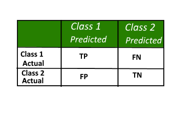
A sample confusion matrix for 2 classes
Definition of the Terms:
• Positive (P): Observation is positive (for example: is a SPAM).• Negative (N): Observation is not positive (for example: is not a SPAM).• True Positive (TP): Observation is positive, and the model predicted positive.• False Negative (FN): Observation is positive, but the model predicted negative.• True Negative (TN): Observation is negative, and the model predicted negative.• False Positive (FP): Observation is negative, but the model predicted positive.
Let us bring two other metrics apart from accuracy which will help us to have a better look at our 3 models
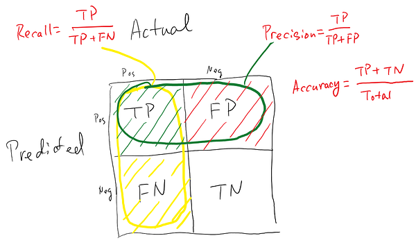
Recall:
The recall is the ratio of the total number of correctly classified positive examples divided to the total number of positive examples. High Recall indicates the class is correctly recognized (small number of FN).
Precision:
To get the value of precision we divide the total number of correctly classified positive examples by the total number of predicted positive examples. High Precision indicates an example labelled as positive is indeed positive (small number of FP).
Let us have a look at the confusion matrix of our SVM classifier and try to understand it. Consecutively, we will be summarising confusion matrix of all our 3 classifiers
Given below is the confusion matrix of the results which our SVM model has predicted on the test data. Let us find out accuracy, precision and recall in this case.

Accuracy = (1446+204)/(1446+3+19+204) = 1650/1672 = 0.986 i.e 98% Accuracy
Recall = (204)/(204+19) = 204/223 = 0.9147 i.e. 91.47% Recall
Precision = (204)(204+3) = 204/207 = 0.985 i.e 98.5% Precision
Understanding the ROC Curve
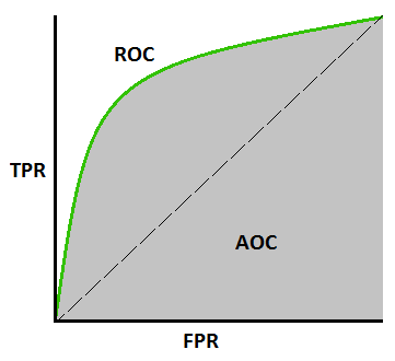
In Machine Learning, performance measurement is an essential task. So when it comes to a classification problem, we can count on an AUC – ROC Curve. It is one of the most important evaluation metrics for checking any classification model’s performance. It is also written as AUROC (Area Under the Receiver Operating Characteristics)
AUC – ROC curve is a performance measurement for classification problem at various thresholds settings. ROC is a probability curve and AUC represents the degree or measure of separability. It tells how much model is capable of distinguishing between classes. Higher the AUC, better the model is at predicting 0s as 0s and 1s as 1s. By analogy, Higher the AUC, better the model is at distinguishing between patients with disease and no disease.
We plot a ROC curve with TPR against the FPR where TPR is on y-axis and FPR is on the x-axis.
Plotting RoC curves for SVM classifier
| from sklearn import metricsprobs = svm.predict_proba(X_test)preds = probs[:,1]fpr, tpr, threshold = metrics.roc_curve(y_test, preds)roc_auc = metrics.auc(fpr, tpr)import matplotlib.pyplot as pltplt.title(‘Receiver Operating Characteristic’)plt.plot(fpr, tpr, ‘b’, label = ‘AUC = %0.2f’ % roc_auc)plt.legend(loc = ‘lower right’)plt.plot([0, 1], [0, 1],’r–‘)plt.xlim([0, 1])plt.ylim([0, 1])plt.ylabel(‘True Positive Rate’)plt.xlabel(‘False Positive Rate’)plt.show() |
probs = svm.predict_proba(X_test)
fpr, tpr, threshold = metrics.roc_curve(y_test, preds)
import matplotlib.pyplot as plt
plt.plot(fpr, tpr, ‘b’, label = ‘AUC = %0.2f’ % roc_auc)
plt.plot([0, 1], [0, 1],’r–’)
plt.ylim([0, 1])
plt.xlabel(‘False Positive Rate’)
Let us have a look at the ROC curve of our SVM classifier
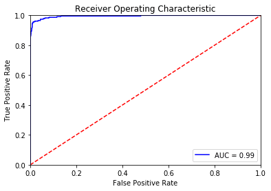
Always remember that the closer AUC (Area under the curve) is to value 1, the better the classification ability of the classifier. Furthermore, let us also have a look at the ROC curve of our KNN and Naive Bayes classifier too!


The graph on the left is for KNN and on the right is for Naive Bayes classifier. This clearly indicates that Naive Bayes classifier, in this case, is much more efficient than our KNN classifier as it has a higher AUC value!
Conclusion
In this series, we looked at understanding NLP from scratch to building our own SPAM classifier over text data. This is an ideal way to start learning NLP as it covers basics of NLP, word embeddings and numeric representations of text data and modeling over those numeric representations. You can also try neural networks for NLP as they are able to achieve good performance! Stay tuned for more on NLP in coming blogs.
Please follow and like us:
![]()