A Thorough Introduction to Boltzmann Machines

The principal task of machine learning is to fit a model to some data. Thinking on the level of APIs, a model is an object with two methods:

Likelihood

How likely is the query point(s) (x) under our model? In other words, how likely was it that our model produced (x)?

The likelihood gives a value proportional to a valid probability, but is not necessarily a valid probability itself.

(Finally, the likelihood is often used as an umbrella term for, or interchangeably with, the probability density. The mainstream machine learning community would do well to agree to the use of one of these terms, and to sunset the other; while their definitions may differ slightly, the confusion brought about by their dual used in almost identical contexts simply does not warrant by the pedagogical purity we maintain by keeping them distinct.

Sample

Draw samples from the model.

Denotation

Canonically, we denote an instance of our Model in mathematical syntax as follows:

x \sim p(x) $$

Again, this simple denotation implies two methods: that we can evaluate the likelihood of having observed (x) under our model (p), and that we can sample a new value (x) from our model (p).

Often, we work with conditional models, such as (y \sim p(y\vert x)), in classification and regression tasks. The same two implicit methods apply.

Boltzmann machines

A Boltzmann machine is one of the simplest mechanisms for modeling (p(x)). It is an undirected graphical model where every dimension (x_i) of a given observation (x) influences every other dimension. As such, we might use it to model data which we believe to exhibit this property, e.g. an image. For (x \in R^3), our model would look as follows:

For (x \in R^n), a given node (x_i) would have (n - 1) outgoing connections in total—one to each of the other nodes (x_j) for (j \neq i).

Finally, a Boltzmann machine strictly operates on binary data. This keeps things simple.

Computing the likelihood

A Boltzmann machines admits the following formula for computing the likelihood of data points (x^{(1)}, …, x^{(n)}):

H(x) = \sum\limits_{i \neq j} w_{i, j} x_i x_j + \sum\limits_i b_i x_i

p(x) = \frac{\exp{(H(x))}}{Z}

\mathcal{L}(x^{(1)}, …, x^{(n)}) = \prod\limits_{i=1}^n p(x^{(i)}) $$

Note:

Since our weights can be negative, (H(x)) can be negative. As a likelihood gives an optionally-normalized probability, it must be non-negative.
To enforce this constraint, we exponentiate (H(x)) in the second equation.
To normalize, we divide by the normalization constant (Z), i.e. the sum of the likelihoods of all possible values of (x^{(1)}, …, x^{(n)}).

Computing the partition function, with examples

In the case of 2-dimensional binary (x), the only possible “configurations” of (x) are: ([0, 0], [0, 1], [1, 0], [1, 1]), i.e. 4 distinct values. This means that in evaluating the likelihood of one datum (x), the normalization constant (Z) would be a sum of 4 terms.

Now, with two data points (x^{(1)}) and (x^{(2)}), there are 16 possible “configurations”:

(x^{(1)} = [0, 0]), (x^{(2)} = [0, 0])
(x^{(1)} = [0, 0]), (x^{(2)} = [0, 1])
(x^{(1)} = [0, 0]), (x^{(2)} = [1, 0])
(x^{(1)} = [0, 0]), (x^{(2)} = [1, 1])
(x^{(1)} = [0, 1]), (x^{(2)} = [0, 0])
(x^{(1)} = [0, 1]), (x^{(2)} = [0, 1])
Etc.

This means that in evaluating the likelihood of (\mathcal{L}(x^{(1)}, x^{(2)})), the normalization constant (Z) would be a sum of 16 terms.

More generally, given (d)-dimensional (x), where each (x_i) can assume one of (v) distinct values, and (n) data points (x^{(1)}, …, x^{(n)})—in evaluating the likelihood of (\mathcal{L}(x^{(1)}, …, x^{(n)})) the normalization constant (Z) would be a sum of ((v^d)^n) terms. With a non-trivially large (v) or (d) (in the discrete case), or a non-trivially large (k) in the continuous case, this becomes intractable to compute.

In the case of a Boltzmann machine, (v = 2), which is not large. Below, we will vary (d) and examine its impact on the tractability (in terms of, “can we actually compute (Z) before the end of the universe?”) of inference.

The likelihood function in code

In code, the likelihood function looks as follows:

This code block is longer than you might expect because it includes a few supplementary behaviors, namely:

Computing the likelihood of one or more points
Avoiding redundant computation of Z
Optionally computing the log-likelihood

Above all, note that: the likelihood is a function of the model’s parameters, i.e. self.weights and self.biases, which we can vary, and the data x, which we can’t.

Training the model

At the outset, the parameters self.weights and self.biases of our model are initialized at random. Trivially, such that the values returned by likelihood and sample are useful, we must first update these parameters by fitting this model to observed data.

To do so, we will employ the principal of maximum likelihood: compute the parameters that make the observed data maximally likely under the model, via gradient ascent.

Gradients

Since our model is simple, we can derive exact gradients by hand. We will work with the log-likelihood instead of the true likelihood to avoid issues of computational underflow. Below, we simplify this expression, then compute its various gradients.

(\log{\mathcal{L}})

\mathcal{L}(x^{(1)}, …, x^{(n)}) = \prod\limits_{k=1}^n \frac{\exp{(H(x^{(k)}))}}{Z}

$\begin{align*} \log{\mathcal{L}(x^{(1)}, ..., x^{(n)})} &= \sum\limits_{k=1}^n \log{\frac{\exp{(H(x^{(k)}))}}{Z}}\\ &= \sum\limits_{k=1}^n \log{\big(\exp{(H(x^{(k)}))}\big)} - \log{Z}\\ &= \sum\limits_{k=1}^n H(x^{(k)}) - \log{Z} \end{align*}$

This gives the total likelihood. Our aim is to maximize the expected likelihood with respect to the data generating distribution.

Expected likelihood

$\begin{align*} \mathop{\mathbb{E}}_{x \sim p_{\text{data}}}\big[ \mathcal{L}(x) \big] &= \sum\limits_{k=1}^N p_{\text{data}}(x = x^{(k)}) \mathcal{L(x^{(k)})}\\ &= \sum\limits_{k=1}^N \frac{1}{N} \mathcal{L(x^{(k)})}\\ &= \frac{1}{N} \sum\limits_{k=1}^N \mathcal{L(x^{(k)})}\\ \end{align*}$

In other words, the average. We will continue to denote this as (\mathcal{L}), i.e. (\mathcal{L} = \frac{1}{N} \sum\limits_{k=1}^n H(x^{(k)}) - \log{Z}).

Now, deriving the gradient with respect to our weights:

(\nabla_{w_{i, j}}\log{\mathcal{L}}):

$\begin{align*} \nabla_{w_{i, j}} \frac{1}{N} \sum\limits_{k=1}^n H(x^{(k)}) - \log{Z} &= \frac{1}{N} \sum\limits_{k=1}^n \nabla_{w_{i, j}} H(x^{(k)}) - \frac{1}{N} \sum\limits_{k=1}^n \nabla_{w_{i, j}} \log{Z} \end{align*}$

First term:

$\begin{align*} \frac{1}{N} \sum\limits_{k=1}^n \nabla_{w_{i, j}} H(x^{(k)}) &= \frac{1}{N} \sum\limits_{k=1}^n \nabla_{w_{i, j}} \sum\limits_{i \neq j} w_{i, j} x_i^{(k)} x_j^{(k)} + \sum\limits_i b_i x_i^{(k)}\\ &= \frac{1}{N} \sum\limits_{k=1}^n x_i^{(k)} x_j^{(k)}\\ &= \mathop{\mathbb{E}}_{x \sim p_{\text{data}}} [x_i x_j] \end{align*}$

Second term:

NB: (\sum\limits_{\mathcal{x}}) implies a summation over all ((v^d)^n) possible configurations of values that (x^{(1)}, …, x^{(n)}) can assume.

$\begin{align*} \nabla_{w_{i, j}} \log{Z} &= \nabla_{w_{i, j}} \log{\sum\limits_{\mathcal{x}}} \exp{(H(x))}\\ &= \frac{1}{\sum\limits_{\mathcal{x}} \exp{(H(x))}} \nabla_{w_{i, j}} \sum\limits_{\mathcal{x}} \exp{(H(x))}\\ &= \frac{1}{Z} \nabla_{w_{i, j}} \sum\limits_{\mathcal{x}} \exp{(H(x))}\\ &= \frac{1}{Z} \sum\limits_{\mathcal{x}} \exp{(H(x))} \nabla_{w_{i, j}} H(x)\\ &= \sum\limits_{\mathcal{x}} \frac{\exp{(H(x))}}{Z} \nabla_{w_{i, j}} H(x)\\ &= \sum\limits_{\mathcal{x}} P(x) \nabla_{w_{i, j}} H(x)\\ &= \sum\limits_{\mathcal{x}} P(x) [x_i x_j]\\ &= \mathop{\mathbb{E}}_{x \sim p_{\text{model}}} [x_i x_j] \end{align*}$

Putting it back together

Combining these constituent parts, we arrive at the following formula:

\nabla_{w_{i, j}}\log{\mathcal{L}} = \mathop{\mathbb{E}}{x \sim p{\text{data}}} [x_i x_j] - \mathop{\mathbb{E}}{x \sim p{\text{model}}} [x_i x_j]

$Finally, following the same logic, we derive the exact gradient with respect to our biases: \nabla_{b_i}\log{\mathcal{L}} = \mathop{\mathbb{E}}_{x \sim p_{\text{data}}} [x_i] - \mathop{\mathbb{E}}_{x \sim p_{\text{model}}} [x_i]$

The first and second terms of each gradient are called, respectively, the positive and negative phases.

Computing the positive phase

In the following toy example, our data are small: we can compute the positive phase using all of the training data, i.e. (\frac{1}{N} \sum\limits_{k=1}^n x_i^{(k)} x_j^{(k)}). Were our data bigger, we could approximate this expectation with a mini-batch of training data and we do in SGD.

Computing the negative phase

Again, this term asks us to compute then sum the log-likelihood over every possible data configuration in the support of our model, which is (O(nv^d)). With non-trivially large (v) or (d), this becomes intractable to compute.

Below, we’ll begin our toy example computing the true negative-phase, (\mathop{\mathbb{E}}{x \sim p{\text{model}}} [x_i x_j]), with varying data dimensionalities (d). Then, once this computation becomes slow, we’ll look to approximate this expectation later on.

Parameter updates in code

Train model, visualize model distribution

Finally, we’re ready to train. Using the true negative phase, let’s train our model for 100 epochs with (d=3) then visualize results.

Train

Visualize samples

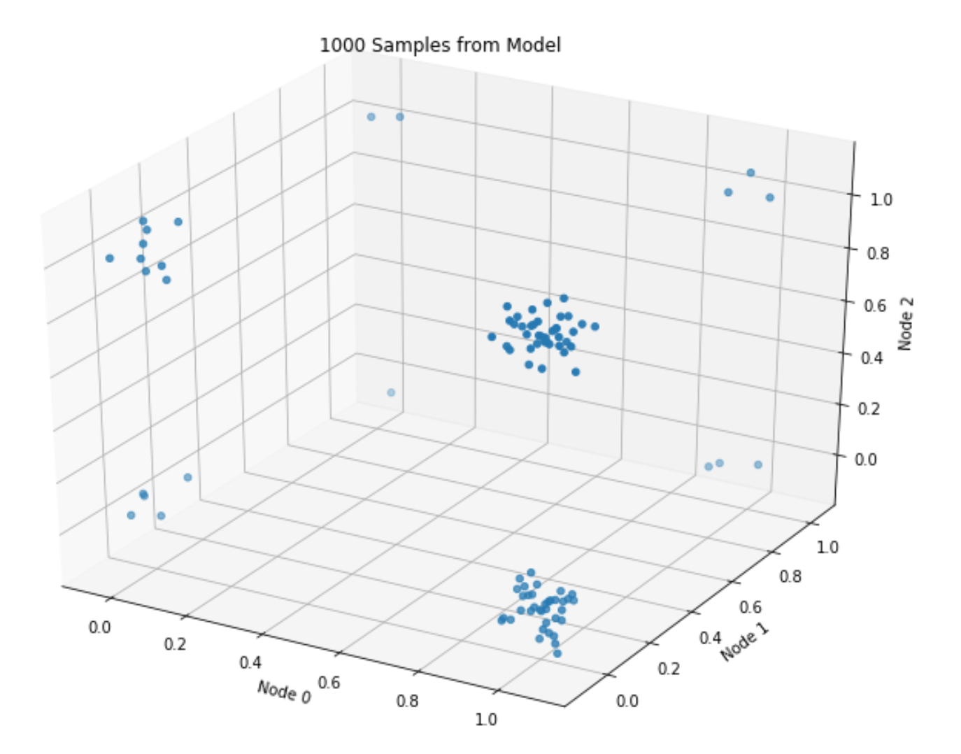
The plot roughly matches the data-generating distribution: most points assume values of either ([1, 0, 1]), or ([1, 0, 0]) (given (p=[.8, .1, .5])).

Sampling, via Gibbs

The second, final method we need to implement is sample. In a Boltzmann machine, we typically do this via Gibbs sampling.

To effectuate this sampling scheme, we’ll need a model of each data dimension conditional on the other data dimensions. For example, for (d=3), we’ll need to define:

(p(x_0\vert x_1, x_2))
(p(x_1\vert x_0, x_2))
(p(x_2\vert x_0, x_1))

Given that each dimension must assume a 0 or a 1, the above 3 models must necessarily return the probability of observing a 1 (where 1 minus this value gives the probability of observing a 0).

Let’s derive these models using the workhorse axiom of conditional probability, starting with the first:

$\begin{align*} p(x_0 = 1\vert x_1, x_2) &= \frac{p(x_0 = 1, x_1, x_2)}{p(x_1, x_2)}\\ &= \frac{p(x_0 = 1, x_1, x_2)}{\sum\limits_{x_0 \in [0, 1]} p(x_0, x_1, x_2)}\\ &= \frac{p(x_0 = 1, x_1, x_2)}{p(x_0 = 0, x_1, x_2) + p(x_0 = 1, x_1, x_2)}\\ &= \frac{1}{1 + \frac{p(x_0 = 0, x_1, x_2)}{p(x_0 = 1, x_1, x_2)}}\\ &= \frac{1}{1 + \frac{\exp{(H(x_0 = 0, x_1, x_2)))}}{\exp{(H(x_0 = 1, x_1, x_2)))}}}\\ &= \frac{1}{1 + \exp{(H(x_0 = 0, x_1, x_2) - H(x_0 = 1, x_1, x_2))}}\\ &= \frac{1}{1 + \exp{(\sum\limits_{i \neq j} w_{i, j} x_i x_j + \sum\limits_i b_i x_i - (\sum\limits_{i \neq j} w_{i, j} x_i x_j + \sum\limits_i b_i x_i))}}\\ &= \frac{1}{1 + \exp{(-\sum\limits_{j \neq i = 0} w_{i, j} x_j - b_i)}}\\ &= \sigma\bigg(\sum\limits_{j \neq i = 0} w_{i, j} x_j + b_i\bigg)\\ \end{align*}$

Pleasantly enough, this model resolves to a simple Binomial GLM, i.e. logistic regression, involving only its neighboring units and the weights that connect them.

With the requisite conditionals in hand, let’s run this chain and compare it with our (trained) model’s true probability distribution.

True probability distribution

Empirical probability distribution, via Gibbs

Close, ish enough.

Scaling up, and hitting the bottleneck

With data of vary dimensionality n_units, the following plot gives the time in seconds that it takes to train this model for 10 epochs.

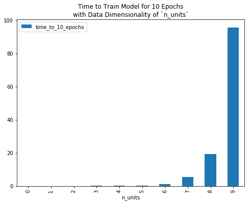
To reduce computational burden, and/or to fit a Boltzmann machine to data of non-trivial dimensionality (e.g. a 28x28 grey-scale image, which implies a random variable with 28x28=784 dimensions), we need to compute the positive and/or negative phase of our gradient faster than we currently are.

To compute the former more quickly, we could employ mini-batches as in canonical stochastic gradient descent.

In this post, we’ll instead focus on ways to speed up the latter. Revisiting its expression, (\mathop{\mathbb{E}}{x \sim p{\text{model}}} [x_i x_j]), we readily see that we can create an unbiased estimator for this value by drawing Monte Carlo samples from our model, i.e.

\mathop{\mathbb{E}}{x \sim p{\text{model}}} [x_i x_j] \approx \frac{1}{N}\sum\limits_{k=1}^N x^{(k)}i x^{(k)}_j\quad\text{where}\quad x^{(k)} \sim p{\text{model}}

So, now we just need a way to draw these samples. Luckily, we have a Gibbs sampler to tap!

Instead of computing the true negative phase, i.e. summing (x_i x_j) over all permissible configurations (X) under our model, we can approximate it by evaluating this expression for a few model samples, then taking the mean.

We define this update mechanism here:

Next, we’ll define a function that we can parameterize by an optimization algorithm (computing the true negative phase, or approximating it via Gibbs sampling, in the above case) which will train a model for (n) epochs and return data requisite for plotting.

How does training progress for varying data dimensionalities?

Finally, for data of n_units 3, 4, 5, etc., let’s train models for 100 epochs and plot likelihood curves.

When training with the approximate negative phase, we’ll:

Derive model samples from a 1000-sample Gibbs chain. Of course, this is a parameter we can tune, which will affect both model accuracy and training runtime. However, we don’t explore that in this post; instead, we just pick something reasonable and hold this value constant throughout our experiments.
Train several models for a given n_units; Seaborn will average results for us then plot a single line (I think).

Plot

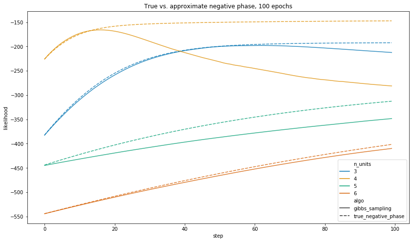
When we let each algorithm run for 100 epochs, the true negative phase gives a model which assigns higher likelihood to the observed data in all of the above training runs.

Notwithstanding, the central point is that 100 epochs of the true negative phase takes a long time to run.

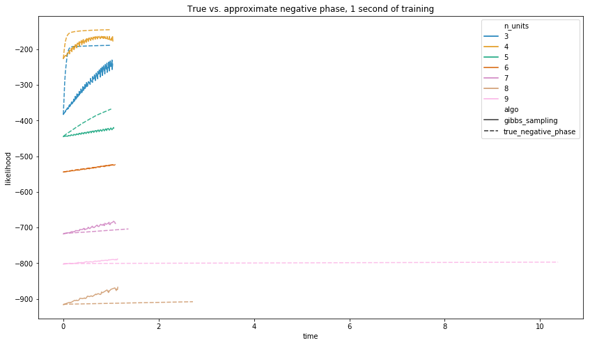
As such, let’s run each for an equal amount of time, and plot results. Below, we define a function to train models for (n) seconds (or 1 epoch—whichever comes first).

How many epochs do we actually get through?

Before plotting results, let’s examine how many epochs each algorithm completes in its allotted time. In fact, for some values of n_units, we couldn’t even complete a single epoch (when computing the true negative phase) in (\leq 1) second.

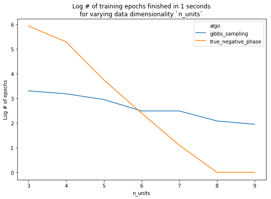
Finally, we look at performance. With n_units <= 7, we see that 1 second of training with the true negative phase yields a better model. Conversely, using 7 or more units, the added performance given by using the true negative phase is overshadowed by the amount of time it takes the model to train.

Plot

Of course, we re-stress that the exact ablation results are conditional (amongst other things) on the number of Gibbs samples we chose to draw. Changing this will change the results, but not that about which we care the most: the overall trend.

Summary

Throughout this post, we’ve given a thorough introduction to a Boltzmann machine: what it does, how it trains, and some of the computational burdens and considerations inherent.

In the next post, we’ll look at cheaper, more inventive algorithms for avoiding the computation of the negative phase, and describe how they’re used in common machine learning models and training routines.

Code

The repository and rendered notebook for this project can be found at their respective links.