By Thomas Tanay
This is a well-known result by now: deep neural networks are vulnerable to tiny perturbations of their inputs [1,2]. In image classification for instance, a dog picture can be slightly altered such that it is recognized as a tabby cat, or a trombone, or any other category for that matter, with high confidence:
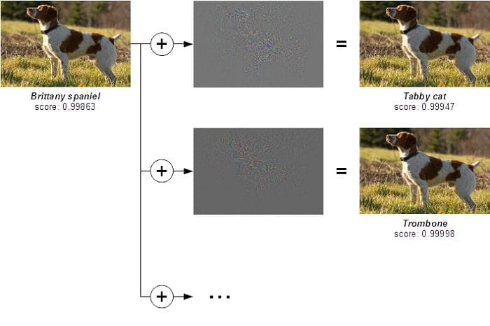
**Fig. 1: Adversarial examples for an inception v3 network trained on ImageNet **
This problem has received considerable research attention in recent years, but it is not going away. In fact, things appear to be worse than initially thought. The phenomenon has for instance been shown to be robust to physical world transformations to some extent, allowing for the construction of 3D objects that are misclassified under a wide distribution of angles and viewpoints [3]. The feasibility of black-box attacks has also been demonstrated, where an attacker is limited to query access without access to internal parameters and gradients [4].
There is an apparent contradiction in the vulnerability of state-of-the-art networks to adversarial examples: how can these models perform so well, if they are so sensitive to small perturbations of their inputs? Think of the feature representations learned: on the one hand, they enable high performance classification and must therefore be highly expressive; on the other hand, they are very fragile and can be altered by small nonsensical noise. Looked at another way, the classes defined in image space appear to be both well-separated and intersecting everywhere. Presumably, this counter-intuitive result has a counter-intuitive origin: perhaps it has to do with the high non-linearity of the models affected? Or with the high dimensionality of the input space?
Consider the distribution of rational numbers in the set of real numbers for a moment. Like the distribution of adversarial examples in image space, it satisfies two properties that are seemingly contradictory: rational numbers are scarce—the vast majority of real numbers are irrational—and yet they are dense—any real interval, however small, contains one. Is it possible that, because of their high non-linearity, deep networks distribute adversarial examples in image space in a similar way: scarcely but densely? The idea has been considered before [1], but it fails to explain a number of experimental results. Most notably, the adversarial example phenomenon is not specific to deep neural networks but affects other machine learning models too, including linear classifiers such as support vector machines (SVMs).
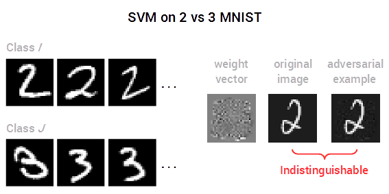
Fig. 2: High non-linearity is not at the origin of the adversarial example phenomenon:linear classifiers are also affected
If high non-linearity is not responsible for the phenomenon, then perhaps high dimensionality is? A number of phenomena that are intuitive in two or three dimensions behave unexpectedly in very high dimension—a problem known as the curse of dimensionality. In this context, the existence of adversarial examples has been argued to be a property of the high-dimensional dot product: “for high-dimensional problems, we can make many infinitesimal changes to the input that add up to one large change to the output” [2]. Yet this explanation is misleading: high-dimensionality can be shown to be neither necessary nor sufficient for the phenomenon to occur.

Fig. 3: High-dimensionality is neither necessary nor sufficient for adversarial examples to exist
In the toy problem above, dimensionality is essentially irrelevant: the classes II and JJ are structurally very similar whether the number of dimensions is 2 or 785. What truly matters is the direction in which the weight vector points. In the low-dimensional example on the left, the weight vector defines a tilted classification boundary that separates classes but lies close to the manifold of normal data. In the high-dimensional example on the right, the classification boundary bisects the classes II and JJ perfectly:

Fig. 4: The manifold of normal data (light and dark blue bars) and the classification boundaries (orange lines) defined by each weight vector in image space
To be precise, the phenomenon of adversarial examples in binary linear classification can always be visualized in a plane of interest—which we call the tilting plane—regardless of the problem considered or the dimensionality of the input space. Formally, the tilting plane is the plane that contains the unit weight vector z^ of the nearest centroid classifier (i.e. the vector passing through the centroids of the two classes) and the weight vector w of the classifier considered; an orthonormal basis (z^,n^) can be found by using the Gram-Schmidt process:
| n=w−(w⋅z^)z^ and n^=n/ | n | . |
. For instance, we can project the training set of the 2 versus 3 MNIST problem considered before in the tilting plane of the weight vector found by SVM. We see that the classification boundary lies close to the data manifold, explaining the vulnerability of this classifier to adversarial examples:

Fig. 5: Projection of the training set of the 2 versus 3 MNIST problem in the tilting plane of the weight vector found by SVM.
Why is the classification boundary tilted in such a way? The short answer is that this is what happens when a linear classifier overfits its training data. In binary linear classification, most of a model’s capacity resides in its ability to tilt with regard to the nearest centroid classifier. When the input space is high dimensional but the data manifold is nearly flat in most directions, as is typically the case with natural images, this capacity can be exploited to separate the training data perfectly, even if the true class distributions are not linearly separable. An important corollary is that it is possible to control the tilting angle of the classification boundary—and therefore its vulnerability to adversarial examples—by using standard regularization techniques designed to reduce overfitting. For instance in the 2 vs 3 MNIST problem, the tilting angle of the SVM boundary depends on the level of L2 regularization used:

Fig. 6: The level of L2 regularization used (slider) controls the tilting angle of theclassification boundary and its vulnerability to adversarial examples.
When regularization is low, the adversarial perturbation is barely perceptible and hard to interpret. When regularization is high however, the adversarial perturbation is clearly visible and simply consists in a difference of centroids. While the first case is counter-intuitive, the second case is hardly surprising; confirming that the existence of adversarial examples in binary linear classification is primarily due to overfitting by boundary tilting.
To understand why the datapoints appear to be moving around when the level of regularization varies in the animation above, one needs to imagine the tilting plane rotating around z^ in input space. This is not easy because the input space is high-dimensional, but the idea can be illustrated in a simplified scenario where the boundary tilts between two positions corresponding to maximum and minimum levels of regularization. In that case, the rotation takes place in the 3D subspace generated by z^ and the two SVM weight vectors of interest, resulting in a clear picture of the phenomenon:

Fig. 7: Tilting of the classification boundary between two positions corresponding to maximum and minimum levels of regularization.Of course, this simple picture does not apply to state-of-the-art deep networks. These models define highly convoluted classification boundaries that cannot be visualized in a single plane. Yet, the study of the binary linear case does contain some helpful insights to tackle this more difficult problem. It shows that the existence of adversarial examples is a non-obvious symptom of overfitting and the role of regularization should be explored further, in accordance with some recent theoretical work [5,6].
References
[1] Intriguing properties of neural networks.
Szegedy, C., et al., 2013. arXiv preprint arXiv:1312.6199.
[2] Explaining and harnessing adversarial examples.
Goodfellow, I., Shlens, J., and Szegedy, C., 2014. arXiv preprint arXiv:1412.6572.
[3] Synthesizing robust adversarial examples.
Athalye, A., and Sutskever, I., 2017. arXiv preprint arXiv:1707.07397.
[4] Query-Efficient Black-box Adversarial Examples.
Andrew, I., et al., 2017. arXiv preprint arXiv:1712.07113.
[5] Adversarially robust generalization requires more data.
Schmidt, L., et al., 2018. arXiv preprint arXiv:1804.11285.
[6] There Is No Free Lunch In Adversarial Robustness (But There Are Unexpected Benefits).
Tsipras, D., et al., 2018. arXiv preprint arXiv:1805.12152.
Bio: Thomas Tanay is a PhD student at CoMPLEX, the centre for mathematics and physics in the life sciences at University College London. He is interested in the limits of deep learning as a model for human vision. In this context, he has recently focused his attention on the counter-intuitive adversarial example phenomenon.
Related: