In today’s blog post we will investigate a practical use case of applying deep learning to hydroponics, a type of method used to grow plants without soil using mineral-rich nutrient solutions in a water solvent.
Specifically, you will learn how to train a Convolutional Neural Network (CNN) using Keras to automatically classify root health without having to physically touch the plants.
The actual experiment design of this tutorial is motivated by Darrah et al. in their 2017 paper, Real- time Root Monitoring of Hydroponic Crop Plants: Proof of Concept for a New Image Analysis System.
Such a system can improve the yields of existing hydroponic farms making farms more efficient and sustainable to run. Of course, the successful application of hydroponics has massive implications for the medical marijuana industry.
While potentially controversial, and knowing full well that I’m going to get a few angry/upset emails about this blog post, I decided to post today’s tutorial anyway.
It’s important, useful, and highly educational for us as students, researchers, and engineers to see practical examples of how deep learning can and is being applied in the real-world.
Furthermore, today’s tutorial is not meant to be a discussion on the legality, morality, or usage of marijuana — this is not a platform to share “Legalize Itâ€� or NORML campaigns, anti-drug campaigns, or simply have a discussion on the recreational use of marijuana. There are more than enough websites on the internet to do that already, and if you feel the need to have such a discussion please do, just understand that PyImageSearch is not that platform.
I’d also urge you to keep in mind that we’re all researchers, students, and developers here, and most importantly, we’re all here to learn from practical, real-world examples. Be civil, regardless of whether you agree or disagree with some of the downstream implications of hydroponics.
With all that said, to learn more about how deep learning is being applied to hydroponics (and yes, medical marijuana), just keep reading!
Deep learning, hydroponics, and medical marijuana
In the first half of today’s blog post, we’ll briefly discuss the concept of hydroponic farms, the relation they have to marijuana, and how deep learning intersects them both.
From there we’ll implement a Convolutional Neural Network with Keras to automatically classify root health of plants grown in a hydroponic system without having to physically touch or interfere with the plant.
Finally, we’ll review the results of our experiment.
What is hydroponics?
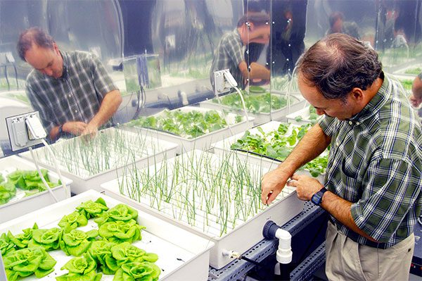
Figure 1: Hydroponic farming is useful to grow and yield more plants within confined spaces. Read the rest of this case study to find out how Keras + deep learning can be used to spot hydroponic root system problem areas.
Hydroponics is a massive industry with an estimated market value of $21,203.5 million USD (yes, million) in 2016. The market is expected to grow at a 6.5% Compound Annual Growth Rate (CAGR) year over year from 2018 to 2023. Europe and Asia are expected to grow at similar rates as well (source for all statistics).
Hydroponics itself is a subset of hydroculture, the process of growing plants without utilizing soil and instead using mineral-rich solutions in a water solvent.
Using hydroponic methods, plants can grow with only their roots touching the mineral solution.
If you automatically correlate the term “hydroponics� with “marijuana�, keep in mind that hydroponic farming has been endorsed and used by major governments and organizations, including the United States, NASA, Europe and even the fabled Hanging Gardens of Babylon.
A great example is the International Space Station (ISS) — we’ve had hydroponic experiments, including growing vegetables, going on at the ISS for years.
Hydroponics is a science that has existed since the Babylonians and Aztecs, and continues to be used in modern times — so before you turn your nose up, keep in mind that this is actual science, and a science far older than computer vision and deep learning.
So, why bother with hydroponic farming at all?
Nutrient soil continues to come at a premium, especially due to irresponsible or over-farming of land, disease, war, deforestation, and an ever-changing environment just to name a few.
Hydroponic farms allow us to grow our fruits and veggies in smaller areas where traditional soil farms may be impossible.
And if you want to consider an even bigger picture, hydroponics will undoubtedly be utilized if we were to ever colonize Mars.
What does hydroponics have to do with medical marijuana?
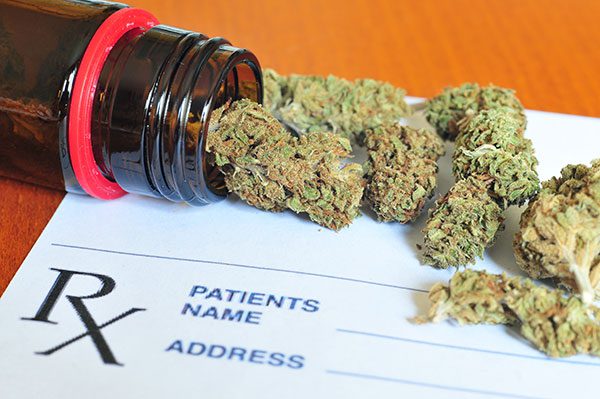
Figure 2: Despite the controversy over the legalization of marijuana in some states in the US, marijuana is often grown via hydroponic means and makes for a great use case of plant root health analysis. Deep learning, by means of the Keras library, is used in this blog post to classify “hairy” (good) vs “non-hairy” (poor) root systems in hydroponics.
If you read the previous section on what hydroponics is and why we use the method, it should come as no surprise that hydroponics is widely used in the marijuana industry, even before legalization legislation (in some states) in the United States.
I’m not going to provide an exhaustive review of hydroponics and medical marijuana (for that, you can refer to this article), but the gist is that:
-
Prior to the legalization of marijuana (in some states of the United States), growers would want to keep their plants secret and safe — growing indoors hydroponically helped with this problem.
-
Medical marijuana rules are new in the United States and in some cases, the only allowed method to grow is hydroponically.
-
Growing hydroponically can help conserve our valuable soil which can take decades or more to naturally replenish itself.
According to reports from the Brightfield Group, the cannabis market was valued at $7.7 billion back in 2017 with a Compound Annual Growth Rate as high as 60% percent as other countries and states legalize — this adds up to a market valuation of $31.4 billion come 2021 (source).
There is a lot of money in hydroponics and marijuana, and in a high-risk, high-reward industry that is inherently dependent on (1) legislation and (2) technology, deep learning has found yet another application.
How do deep learning, computer vision, and hydroponics intersect?
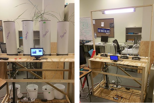
Figure 3: PyImageSearch reader, Timothy Darrah’s research lab for analyzing plant root health in a hydroponics growing configuration is pictured with his permission. His project inspired this deep learning blog post.
Back in 2017, PyImageSearch reader Timothy Darrah, an undergraduate at Tennessee State University, reached out to me with an interesting problem — he needed to devise an algorithm to automatically classify plant roots without being able to touch or interfere with the plants in anyway.
In particular, Darrah was working with switchgrass plants, a dominant species of North American prairie grass.
Note: Darrah et al.’s work was published in a paper entitled Real- time Root Monitoring of Hydroponic Crop Plants: Proof of Concept for a New Image Analysis System. Darrah has graciously allowed me to host his paper for your viewing.
The overall goal of the project was to develop an automated root growth analysis system capable of accurately measuring the roots followed by detecting any growth problems:
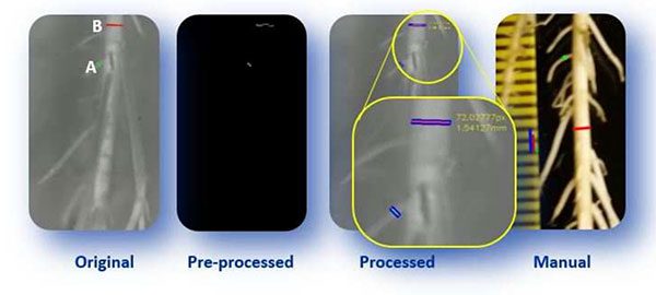
Figure 4: An automated root growth analysis system concept. We’re demonstrating the concept of deep learning as a tool to help classify the roots in a hydroponic system.
In particular, roots needed to be classified into two groups:
-
“Hairy� roots
-
“Non-hairy� roots
The “hairier� a root is, the better the root can suck up nutrients.
The “less hairy” the root is, the fewer nutrients it can intake, potentially leading to the plant starving and dying.
For this project, Timothy, along with Mahesh Rangu (a Ph.D. student) and their advisors, Dr. Erdem Erdemir and Dr. Suping Zhou, developed a system to automatically capture root images without having to disturb the plant itself.
Example images of their experimental setup can be seen in Figure 3 at the top of this section.
From there, they needed to apply computer vision to classify the root into one of the two categories (and eventually multiple categories for detecting other root afflictions).
The only question was how to solve the image classification problem?
Note: Timothy and the rest of the team solved their initial problem after Timothy emailed me in April 2017 asking for an algorithm to try. I suggested Local Binary Patterns which worked for them; however, for the sake of this tutorial, we’ll explore how deep learning can be utilized as well.
Our image dataset
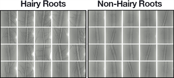
Figure 5: Our deep learning dataset for hydroponics root analysis.
Our dataset of 1,524 root images includes:
-
Hairy: 748 images (left)
-
Non-hairy: 776 images (right)
A subset of the example images for each class can be seen in Figure 4 above.
The original images were captured at a higher resolution of 1920×1080 pixels; however, for the sake for this blog post, I’ve resized them to 256×256 pixels as a matter of convenience (and to save space/bandwidth).
The resizing was performed by:
-
Resizing the height to 256 pixels
-
And then taking the center 256-pixel crop
Since the center of the image always contained the mass of root hairs (or lack thereof), this resizing and cropping method worked quite well.
Darrah et al. have graciously allowed us to use these images for our own education as well (but you cannot use them for commercial purposes).
In the remainder of this tutorial, you will learn how to train a deep learning network to automatically classify each of these root species classes.
Project structure
To review the project structure directly in your terminal, first, grab the “Downloads” for this post and unzip the archive.
Then navigate into the project directory and use the tree command to examine the contents:
| $ tree –dirsfirst –filelimit 10.├── dataset│ ├── hairy_root [748 images]│ └── non_hairy_root [776 images]├── pyimagesearch│ ├── init.py│ └── simplenet.py├── train_network.py└── plot.png 4 directories, 4 files |
.
│ ├── hairy_root [748 images]
├── pyimagesearch
│ └── simplenet.py
└── plot.png
4 directories, 4 files
Our dataset/ directory consists of hairy_root/ and non_hairy_root/ images.
The pyimagesearch/ directory is a Python module containing simplenet.py . The SimpleNet architecture is a Keras deep learning architecture I designed for root health classification. We’ll be reviewing this architecture today.
We’ll then train our network with train_network.py , producing plot.png , our training plot. We’ll walk through the training script line by line so you have an understanding of how it works.
Let’s begin!
Utilizing deep learning to classify root health
Now that we have an understanding of both (1) hydroponics and (2) the dataset we are working with, we can get started.
Installing necessary software
For today’s case study, you’ll need the following software installed on your computer:
-
OpenCV: Any version will work for today’s example as we are just taking advantage of its basic functionality. Visit my OpenCV Tutorials, Resources, and Guides and select the install tutorial appropriate for your system.
-
Keras and TensorFlow: See Installing Keras with TensorFlow backend to get started. Take note of the name of the Python virtual environment you installed OpenCV into — you’ll want to use the same environment to install Keras and TF in.
scikit-learn: Easily install into your virtual environment with pip: pip install scikit-learn . imutils: My package of convenience functions for image processing can be installed via pip install imutils . matplotlib: A plotting tool for Python — pip install matplotlib .
Implementing our Convolutional Neural Network
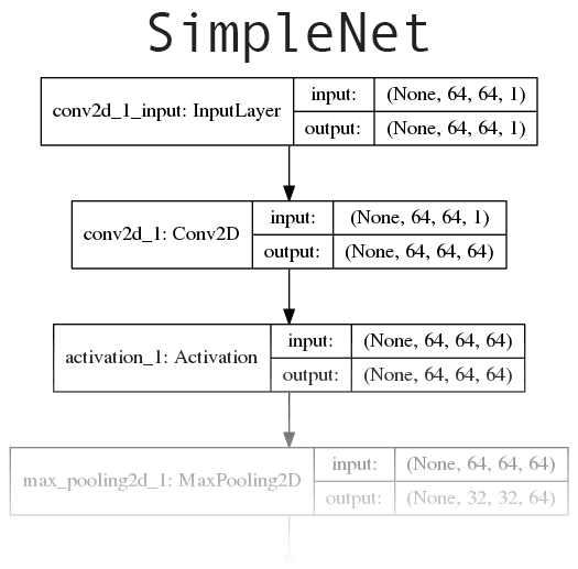
Figure 6: Our deep learning Convolutional Neural Network (CNN) is based on the concepts of AlexNet and OverFeat. Keras will be utilized to build the network and train the model. We will apply this CNN to hydroponics root analysis where marijuana growers might take notice as hydroponics accounts for a segment of their agriculture industry.
The network we’ll be implementing today is loosely based on concepts introduced in AlexNet and OverFeat.
Our network will start off with convolutional filters with a larger filter size used to quickly reduce the spatial dimensions of the volume. From there we’ll apply two CONV layers used to learn 3×3 filters. Click here to see the full network architecture diagram.
Open up the simplenet.py file and insert the following code:
| # import the necessary packagesfrom keras.models import Sequentialfrom keras.layers.convolutional import Conv2Dfrom keras.layers.convolutional import MaxPooling2Dfrom keras.layers.core import Activationfrom keras.layers.core import Flattenfrom keras.layers.core import Dropoutfrom keras.layers.core import Densefrom keras import backend as K |
from keras.models import Sequential
from keras.layers.convolutional import MaxPooling2D
from keras.layers.core import Flatten
from keras.layers.core import Dense
We begin our script by importing necessary layer types from keras . Scroll down to see each in use.
We also import the keras backend . The backend will allow us to dynamically handle different input shapes in the next block where we define the SimpleNet class and build method:
| class SimpleNet: @staticmethod def build(width, height, depth, classes, reg): # initialize the model along with the input shape to be # “channels last” model = Sequential() inputShape = (height, width, depth) # if we are using “channels first”, update the input shape if K.image_data_format() == “channels_first”: inputShape = (depth, height, width) |
@staticmethod
# initialize the model along with the input shape to be
model = Sequential()
if K.image_data_format() == “channels_first”:
The SimpleNet class definition begins on Line 11.
Our only method, build , is defined on Line 13.
The first step in the function is to initialize a Sequential model (Line 16).
Then we specify our inputShape where input images are assumed to be 64×64 pixels in size (Line 17).
Most people will be using TensorFlow as the backend which assumes “channels_last” last ordering. In case you are using Theano or another “channels_first” backend, then the inputShape is modified on Lines 20 and 21.
Let’s begin adding layers to our network:
| 2324252627282930313233343536373839404142 | # first set of CONV => RELU => POOL layers model.add(Conv2D(64, (11, 11), input_shape=inputShape, padding=”same”, kernel_regularizer=reg)) model.add(Activation(“relu”)) model.add(MaxPooling2D(pool_size=(2, 2))) model.add(Dropout(0.25)) # second set of CONV => RELU => POOL layers model.add(Conv2D(128, (5, 5), padding=”same”, kernel_regularizer=reg)) model.add(Activation(“relu”)) model.add(MaxPooling2D(pool_size=(2, 2))) model.add(Dropout(0.25)) # third (and final) CONV => RELU => POOL layers model.add(Conv2D(256, (3, 3), padding=”same”, kernel_regularizer=reg)) model.add(Activation(“relu”)) model.add(MaxPooling2D(pool_size=(2, 2))) model.add(Dropout(0.25)) |
24
26
28
30
32
34
36
38
40
42
model.add(Conv2D(64, (11, 11), input_shape=inputShape,
model.add(Activation(“relu”))
model.add(Dropout(0.25))
# second set of CONV => RELU => POOL layers
kernel_regularizer=reg))
model.add(MaxPooling2D(pool_size=(2, 2)))
model.add(Conv2D(256, (3, 3), padding=”same”,
model.add(Activation(“relu”))
model.add(Dropout(0.25))
The first CONV => RELU => POOL block of layers (Lines 24-28) uses a larger filter size to (1) help detect larger groups of hairs (or lack thereof), followed by (2) quickly reducing the spatial dimensions of the volume.
We learn more filters per CONV layer the deeper in the network we go (Lines 31-42).
Standard Rectified Linear Unit (RELU) activation is utilized throughout. Alternatives and tradeoffs are discussed in my deep learning book.
POOL layers have a primary function of progressively reducing the spatial size (i.e. width and height) of the input volume to a layer. You’ll commonly see POOL layers between consecutive CONV layers in a CNN such as this example.
In each of the blocks above, we dropout 25% of the nodes (disconnect random neurons) in an effort to introduce regularization and help the network generalize better. This method is proven to reduce overfitting, increase accuracy, and allow our network to generalize better for unfamiliar images.
Our last FC => RELU block ends with a softmax classifier:
| # first and only set of FC => RELU layers model.add(Flatten()) model.add(Dense(512, kernel_regularizer=reg)) model.add(Activation(“relu”)) model.add(Dropout(0.5)) # softmax classifier model.add(Dense(classes)) model.add(Activation(“softmax”)) # return the constructed network architecture return model |
model.add(Flatten())
model.add(Activation(“relu”))
model.add(Dense(classes))
return model
Fully connected layers ( Dense ) are common towards the end of CNNs. This time we apply 50% dropout.
Our softmax classifier is applied to our last fully connected layer which has 2 outputs corresponding to our two classes : (1) non_hairy_root , and (2) hairy_root .
Finally, we return the constructed model.
Implementing the driver script
Now that we’ve implemented SimpleNet , let’s create the driver script responsible for training our network.
Open up train_network.py and insert the following code:
| 12345678910111213141516171819 | # set the matplotlib backend so figures can be saved in the backgroundimport matplotlibmatplotlib.use(“Agg”) # import the necessary packagesfrom pyimagesearch.simplenet import SimpleNetfrom sklearn.preprocessing import LabelEncoderfrom sklearn.model_selection import train_test_splitfrom sklearn.metrics import classification_reportfrom keras.optimizers import Adamfrom keras.regularizers import l2from keras.utils import np_utilsfrom imutils import build_montagesfrom imutils import pathsimport matplotlib.pyplot as pltimport numpy as npimport argparseimport cv2import os |
2
4
6
8
10
12
14
16
18
import matplotlib
from pyimagesearch.simplenet import SimpleNet
from sklearn.model_selection import train_test_split
from keras.optimizers import Adam
from keras.utils import np_utils
from imutils import paths
import numpy as np
import cv2
Our driver script has a number of important imports. Let’s review them:
matplotlib : The de facto plotting package for Python. We’ll be plotting our training accuracy/loss data over time.
SimpleNet : We defined this CNN architecture in the previous section.
LabelEncoder : The scikit-learn package has a handy label encoder. We’ll perform “one-hot” encoding — more on that later.
train_test_split : We’re going to segment our training data into a certain percentage of images for training and the remaining images for testing. Splitting data is common in machine learning and you’ll find a similar function no matter what tool you are using.
classification_report : Allows us to conveniently print statistics in a readable format in our terminal.
Adam : A learning optimizer that we’ll be using. Another option would have been SGD.
l2 : Incorporated into the loss function, the l2 regularizer allows us to penalize layer parameters or layer activity during optimization. This will prevent overfitting and allow our network to generalize.
build_montages : We’ll view the results of our hard work in a montage of images within one frame. This comes from my imutils package.
paths : Also from imutils, this function will extract all image paths (recursively) from an input directory.
argparse : For parsing command line arguments — we’ll review this next.
cv2 : Don’t forget about OpenCV! We’ll use OpenCV for preprocessing as well as visualization/display.
os : I’m not a Windows guy, nor do I officially support Windows here on PyImageSearch, but we’ll use os.path.sep which will accommodate Windows and Linux/Mac path separators.
That was a mouthful. The more you work in the field of CV and DL, the more familiar you’ll become with these and other packages and modules.
Let’s take advantage of one of them. We’ll use argparse to parse our command line arguments:
| # construct the argument parser and parse the argumentsap = argparse.ArgumentParser()ap.add_argument(“-d”, “–dataset”, required=True, help=”path to input dataset”)ap.add_argument(“-e”, “–epochs”, type=int, default=100, help=”# of epochs to train our network for”)ap.add_argument(“-p”, “–plot”, type=str, default=”plot.png”, help=”path to output loss/accuracy plot”)args = vars(ap.parse_args()) |
ap = argparse.ArgumentParser()
help=”path to input dataset”)
help=”# of epochs to train our network for”)
help=”path to output loss/accuracy plot”)
Readers of my blog tend to be familiar with these lines of code, but I always explain them for newcomers. The argparse tool will parse a command string entered in your terminal with command line arguments. Be sure to read my post on Python, argparse, and command line arguments if it is your first time here or if you’ve never used command line arguments before.
We have three command line arguments for our driver script:
–dataset : This is the path to our dataset of images. This argument is required as we need data for training.
–epochs : You can experiment with training for different numbers of iterations (epochs). I found 100 to be adequate, so it is the default.
–plot : If you’d like to specify a path + filename for your plot, you can do so with this argument. By default, your plot will be named “plot.png” and saved in the current working directory. Each time you run an experiment with a goal of better performance, you should make note of DL parameters and also name your plot so you’ll remember which experiment it corresponds to.
Now that we’ve parsed our command line arguments, let’s load + preprocess our image data and parse labels:
| 313233343536373839404142434445464748495051 | # grab the list of images in our dataset directory, then initialize# the list of data (i.e., images) and class imagesprint(“[INFO] loading images…“)imagePaths = list(paths.list_images(args[“dataset”]))data = []labels = [] # loop over the image pathsfor imagePath in imagePaths: # extract the class label from the filename label = imagePath.split(os.path.sep)[-2] # load the image, convert it to grayscale, and resize it to be a # fixed 64x64 pixels, ignoring aspect ratio image = cv2.imread(imagePath) image = cv2.cvtColor(image, cv2.COLOR_BGR2GRAY) image = cv2.resize(image, (64, 64)) # update the data and labels lists, respectively data.append(image) labels.append(label) |
32
34
36
38
40
42
44
46
48
50
the list of data (i.e., images) and class images
imagePaths = list(paths.list_images(args[“dataset”]))
labels = []
loop over the image paths
# extract the class label from the filename
# fixed 64x64 pixels, ignoring aspect ratio
image = cv2.cvtColor(image, cv2.COLOR_BGR2GRAY)
data.append(image)
On Line 34 we create a list of all imagePaths in our dataset. We then go ahead and initialize a place to hold our data in memory as well as our corresponding labels (Lines 35 and 36).
Given our imagePaths , we proceed to loop over them on Line 39.
The first step in the loop is to extract our class label on Line 41. Let’s see how this works in a Python Shell:
| $ python»> from imutils import paths»> import os»> imagePaths = list(paths.list_images(“dataset”))»> imagePath = imagePaths[0]»> imagePath’dataset/hairy_root/100_a.jpg’»> imagePath.split(os.path.sep)[‘dataset’, ‘hairy_root’, ‘100_a.jpg’]»> imagePath.split(os.path.sep)[-2]’hairy_root’»> |
from imutils import paths
imagePaths = list(paths.list_images(“dataset”))
imagePath
imagePath.split(os.path.sep)
imagePath.split(os.path.sep)[-2]
Notice how by using imagePath.split and providing the split character (the OS path separator — “/” on Unix and “\” on Windows), the function produces a list of folder/file names (strings) which walk down the directory tree (Lines 8 and 9). We grab the second-to-last index, the class label, which in this case is ‘hairy_root’ (Lines 10 and 11).
Then we proceed to load the image and preprocess it (Lines 45-47). Grayscale (single channel) is all we need to identify hairy or non-hairy roots. Our network requires 64×64 pixel images by design.
Finally, we add the image to data and the label to labels (Lines 50 and 51).
Next, we’ll reshape our data and encode labels:
| 53545556575859606162636465666768697071727374 | # convert the data into a NumPy array, then preprocess it by scaling# all pixel intensities to the range [0, 1]data = np.array(data, dtype=”float”) / 255.0 # reshape the data matrix so that it explicity includes a channel# dimensiondata = data.reshape((data.shape[0], data.shape[1], data.shape[2], 1)) # encode the labels (which are currently strings) as integersle = LabelEncoder()labels = le.fit_transform(labels) # transform the labels into vectors in the range [0, classes],# generating a vector for each label, where the index of the label# is set to ‘1’ and all other entries are set to ‘0’ – this process# is called “one-hot encoding”labels = np_utils.to_categorical(labels, 2) # partition the data into training and testing splits using 60% of# the data for training and the remaining 40% for testing(trainX, testX, trainY, testY) = train_test_split(data, labels, test_size=0.40, stratify=labels, random_state=42) |
54
56
58
60
62
64
66
68
70
72
74
all pixel intensities to the range [0, 1]
dimension
le = LabelEncoder()
generating a vector for each label, where the index of the label
is called “one-hot encoding”
the data for training and the remaining 40% for testing
test_size=0.40, stratify=labels, random_state=42)
Data is reshaped on Lines 55-59. During the process, we convert from a list to a NumPy array of floats that are scaled to [0, 1]. We also add the channel dimension even though we have only one grayscale channel. This extra dimension is expected by our CNN.
We then encode our labels on Lines 62-69. We use “one-hot encoding” which implies that we have a vector where only one of the elements (classes) is “hot” at any given time. Review my recent Keras tutorial for an example applied to a dataset of 3 classes to grasp the concept.
Now comes the splitting of the data. I’ve reserved 60% of our data for training and 40% for testing (Lines 73 and 74).
Let’s compile our model:
| # initialize the optimizer and modelprint(“[INFO] compiling model…“)opt = Adam(lr=1e-4, decay=1e-4 / args[“epochs”])model = SimpleNet.build(width=64, height=64, depth=1, classes=len(le.classes_), reg=l2(0.0002))model.compile(loss=”binary_crossentropy”, optimizer=opt, metrics=[“accuracy”]) |
print(“[INFO] compiling model…”)
model = SimpleNet.build(width=64, height=64, depth=1,
model.compile(loss=”binary_crossentropy”, optimizer=opt,
We initialize the Adam optimizer with a learning rate of 1e-4 and learning rate decay (Line 78).
Note:**The default learning rate for Adam is 1e-3 , but I found through experimentation that using 1e-3 was too high — the network was unable to gain any “traction” and unable to learn. Using 1e-4 as the initial learning rate allowed the network to start learning. This goes to show you how important it is to understand deep learning parameters and fundamentals. Grab a copy of my book, Deep Learning for Computer Vision with Python, to discover my best practices, tips, and suggestions when tuning these parameters.
I also included a small amount of regularization to help prevent overfitting and ensure the network generalizes. This regularization is shown on Lines 79 and 80 where we build our model while specifying our dimensions, encoded labels, as well as the regularization strength.
We compile our model on Lines 81 and 82. Since our network has only two classes, we use “binary_crossentropy” . If you have > 2 classes, you would want to use “categorical_crossentropy” .
Training is kicked off next, followed by evaluation:
| # train the networkprint(“[INFO] training network for {} epochs…“.format( args[“epochs”]))H = model.fit(trainX, trainY, validation_data=(testX, testY), batch_size=32, epochs=args[“epochs”], verbose=1) # evaluate the networkprint(“[INFO] evaluating network…“)predictions = model.predict(testX, batch_size=32)print(classification_report(testY.argmax(axis=1), predictions.argmax(axis=1), target_names=le.classes_)) |
print(“[INFO] training network for {} epochs…“.format(
H = model.fit(trainX, trainY, validation_data=(testX, testY),
print(“[INFO] evaluating network…”)
print(classification_report(testY.argmax(axis=1),
Training, also known as “fitting a model” is kicked off on Lines 87 and 88. I’ve set a batch size of 32 .
We then evaluate the network and print a classification_report in the terminal (Lines 92-94).
Next, we use matplotlib to generate a training plot:
| 96979899100101102103104105106107108 | # plot the training loss and accuracyN = args[“epochs”]plt.style.use(“ggplot”)plt.figure()plt.plot(np.arange(0, N), H.history[“loss”], label=”train_loss”)plt.plot(np.arange(0, N), H.history[“val_loss”], label=”val_loss”)plt.plot(np.arange(0, N), H.history[“acc”], label=”train_acc”)plt.plot(np.arange(0, N), H.history[“val_acc”], label=”val_acc”)plt.title(“Training Loss and Accuracy on Dataset”)plt.xlabel(“Epoch #”)plt.ylabel(“Loss/Accuracy”)plt.legend(loc=”lower left”)plt.savefig(args[“plot”]) |
97
99
101
103
105
107
N = args[“epochs”]
plt.figure()
plt.plot(np.arange(0, N), H.history[“val_loss”], label=”val_loss”)
plt.plot(np.arange(0, N), H.history[“val_acc”], label=”val_acc”)
plt.xlabel(“Epoch #”)
plt.legend(loc=”lower left”)
The above is a good recipe to refer to for producing a training plot when working with Keras and deep learning. The code plots loss and accuracy on the same plot (y-axis) throughout the training period (x-axis).
We call savefig to export the plot image to disk (Line 108).
Finally, let’s visualize the output:
| 110111112113114115116117118119120121122123124125126127128129130131132133134135136137138139140141142 | # randomly select a few testing images and then initialize the output# set of imagesidxs = np.arange(0, testY.shape[0])idxs = np.random.choice(idxs, size=(25,), replace=False)images = [] # loop over the testing indexesfor i in idxs: # grab the current testing image and classify it image = np.expand_dims(testX[i], axis=0) preds = model.predict(image) j = preds.argmax(axis=1)[0] label = le.classes_[j] # rescale the image into the range [0, 255] and then resize it so # we can more easily visualize it output = (image[0] * 255).astype(“uint8”) output = np.dstack([output] * 3) output = cv2.resize(output, (128, 128)) # draw the colored class label on the output image and add it to # the set of output images label_color = (0, 0, 255) if “non” in label else (0, 255, 0) cv2.putText(output, label, (3, 20), cv2.FONT_HERSHEY_SIMPLEX, 0.5, label_color, 2) images.append(output) # create a montage using 128x128 “tiles” with 5 rows and 5 columnsmontage = build_montages(images, (128, 128), (5, 5))[0] # show the output montagecv2.imshow(“Output”, montage)cv2.waitKey(0) |
111
113
115
117
119
121
123
125
127
129
131
133
135
137
139
141
set of images
idxs = np.random.choice(idxs, size=(25,), replace=False)
for i in idxs:
image = np.expand_dims(testX[i], axis=0)
j = preds.argmax(axis=1)[0]
# we can more easily visualize it
output = np.dstack([output] * 3)
# the set of output images
cv2.putText(output, label, (3, 20), cv2.FONT_HERSHEY_SIMPLEX, 0.5,
images.append(output)
create a montage using 128x128 “tiles” with 5 rows and 5 columns
cv2.imshow(“Output”, montage)
Whenever you are testing a machine learning or deep learning model, you shouldn’t only rely on statistics as proof that the model is working. You should also visualize your results on test images. Sometimes I make a separate script which loads an arbitrary image and classifies + displays it. Given that these images are all similar, I opted to make a montage of images so we can visually check at a glance if our model is performing well.
The steps to do this include:
Randomly select some testing image indexes to visualize (Lines 112 and 113). Also initialize a list to hold the images (Line 114). Loop over the random image idxs beginning on Line 117:
Load and classify the image (Lines 119-122). We take the index of the highest prediction and feed the index to our label encoder to generate a label .
- Rescale/resize the image for visualization (Lines 126-128).
Draw the label text on the output image (Lines 132-134). The hairy roots (good) will have green font and non-hairy roots (bad) will be red. Add the output image to our images list so that we can later build a montage (Line 135).
Finally, we display the results until a key is pressed on the final two lines.
Root health classification results
To see how our root health deep neural network performed, be sure to use the “Downloads� section of this blog post to download the source code and dataset.
From there, open up a terminal, navigate to where you downloaded + extracted the code, and execute the following command:
| 1234567891011121314151617181920212223242526 | $ python train_network.py –dataset datasetUsing TensorFlow backend.[INFO] loading images…[INFO] compiling model…[INFO] training network for 100 epochs…Train on 914 samples, validate on 610 samplesEpoch 1/100914/914 [==============================] - 2s - loss: 0.9463 - acc: 0.5022 - val_loss: 0.9245 - val_acc: 0.8000Epoch 2/100914/914 [==============================] - 1s - loss: 0.9188 - acc: 0.5120 - val_loss: 0.9074 - val_acc: 0.7705Epoch 3/100914/914 [==============================] - 1s - loss: 0.9020 - acc: 0.4978 - val_loss: 0.8923 - val_acc: 0.6705…Epoch 98/100914/914 [==============================] - 1s - loss: 0.1212 - acc: 0.9836 - val_loss: 0.1013 - val_acc: 0.9951Epoch 99/100914/914 [==============================] - 1s - loss: 0.0965 - acc: 0.9945 - val_loss: 0.1017 - val_acc: 0.9918Epoch 100/100914/914 [==============================] - 1s - loss: 0.1005 - acc: 0.9891 - val_loss: 0.1040 - val_acc: 0.9902[INFO] evaluating network… precision recall f1-score support hairy_root 1.00 0.98 0.99 299non_hairy_root 0.98 1.00 0.99 311 avg / total 0.99 0.99 0.99 610 |
2
4
6
8
10
12
14
16
18
20
22
24
26
Using TensorFlow backend.
[INFO] compiling model…
Train on 914 samples, validate on 610 samples
914/914 [==============================] - 2s - loss: 0.9463 - acc: 0.5022 - val_loss: 0.9245 - val_acc: 0.8000
914/914 [==============================] - 1s - loss: 0.9188 - acc: 0.5120 - val_loss: 0.9074 - val_acc: 0.7705
914/914 [==============================] - 1s - loss: 0.9020 - acc: 0.4978 - val_loss: 0.8923 - val_acc: 0.6705
Epoch 98/100
Epoch 99/100
Epoch 100/100
[INFO] evaluating network…
non_hairy_root 0.98 1.00 0.99 311
avg / total 0.99 0.99 0.99 610
 Figure 7: Our deep learning training plot contains accuracy and loss curves for our hydroponics plant root health case study. The CNN was trained with Keras and the plot was generated with Matplotlib.
As we can see, our network obtained 99% classification accuracy, and as our plot demonstrates, there is no overfitting.
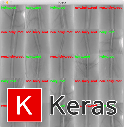
And furthermore, we can examine the montage of our results which again show that our network is accurately classifying each of the root types:
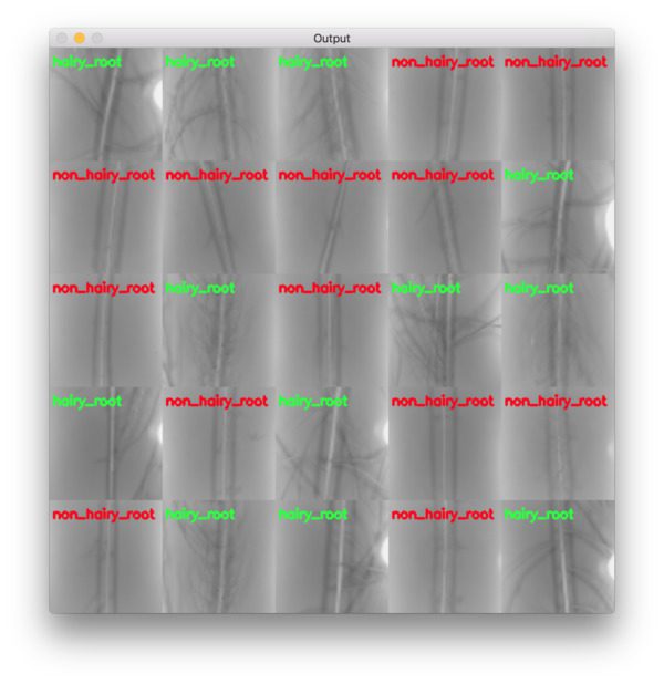
Figure 8: A montage of our hydroponic root classification system results. Keras + deep learning was utilized to build a “hairy_root” vs “non_hairy_root” classifier. Training images were provided by Darrah et al.’s research.
Using techniques such as this one, deep learning researchers, practitioners, and engineers can help solve real-world problems.
Summary
In today’s blog post we explored a real-world application of deep learning: automatically classifying plant root health in hydroponic farms, and in particular, how such a system could be leveraged in the massively growing (no pun intended) medical marijuana industry.
In order to classify root health, we trained a Convolutional Neural Network with Keras and Python to label roots as “hairy� or “non-hairy�.
The more hairs a root has, the more easily it is able to intake nutrients. The fewer hairs a root has, the more it will struggle to suck up nutrients, potentially leading to the plant dying and the loss of the crop.
Using the method detailed in today’s post we were able to classify root health with over 99% accuracy.
For more information on how hydroponics and computer vision intersect, please refer to Darrah et al.’s 2017 publication.
I hope you enjoyed today’s blog post on applying deep learning to a real-world application.
To download the source code to this blog post (and signup for the PyImageSearch newsletter), just enter your email address in the form below!