Should I be using Keras vs. TensorFlow for my project? Is TensorFlow or Keras better? Should I invest my time studying TensorFlow? Or Keras?

The above are all examples of questions I hear echoed throughout my inbox, social media, and even in-person conversations with deep learning researchers, practitioners, and engineers.

I even receive questions related to my book, Deep Learning for Computer Vision with Python where readers are asking why Iâ€™m covering â€œjustâ€� Keras — what about TensorFlow?

Itâ€™s unfortunate.

Because it’s the wrong question to be asking.

As of mid-2017, Keras was actually fully adopted and integrated into TensorFlow. This TensorFlow + Keras integration means that you can:

Define your model using the easy to use interface of Keras
And then drop down into TensorFlow if you need (1) specific TensorFlow functionality or (2) need to implement a custom feature that Keras does not support but TensorFlow does.

In short:

You can insert TensorFlow code directly into your Keras model or training pipeline!

Donâ€™t get me wrong. Iâ€™m not saying that you donâ€™t need to understand a bit of TensorFlow for certain applications â€” this is especially true if youâ€™re performing novel research and need custom implementations. Iâ€™m just saying that if youâ€™re spinning your wheels:

Just getting started studying deep learning…
Trying to decide on which library to use for your next project…
Wondering if Keras or TensorFlow is â€œbetterâ€�…

…then itâ€™s time those wheels got some traction.

Stop worrying and just get started. My suggestion would be to use Keras to start and then drop down into TensorFlow for any specific functionality you may need.

In todayâ€™s post, Iâ€™ll show you how you can train both (1) a neural network using strict Keras and (2) a model using the Keras + TensorFlow integration (with custom features) built directly into the TensorFlow library.

To learn more about Keras vs. Tensorflow, just keep reading!

Keras vs. TensorFlow – Which one is better and which one should I learn?

In the remainder of todayâ€™s tutorial, Iâ€™ll continue to discuss the Keras vs. TensorFlow argument and how itâ€™s the wrong question to be asking.

From there weâ€™ll implement a Convolutional Neural Network (CNN) using both the standard keras module along with the tf.keras module baked right into TensorFlow.

Weâ€™ll train these CNNs on an example dataset and then examine the results â€” as youâ€™ll find out, Keras and TensorFlow live together in harmony.

And perhaps most importantly, youâ€™ll learn why the Keras vs. TensorFlow argument doesnâ€™t make much sense anymore.

If youâ€™re asking â€œKeras vs. TensorFlowâ€�, youâ€™re asking the wrong question

Figure 1: “Should I use Keras or Tensorflow?”

Asking whether you should be using Keras or TensorFlow is the wrong question — and in fact, the question doesnâ€™t even make sense anymore. Even though itâ€™s been over a year since TensorFlow announced that Keras will be integrated into official TensorFlow releases, Iâ€™m still surprised by the number of deep learning practitioners who are unaware that they can access Keras via the tf.keras sub-module.

And more to the point — that the Keras + TensorFlow integration is seamless, allowing you to drop raw TensorFlow code directly into your Keras model.

Using Keras inside of TensorFlow gives you the best of both worlds:

You can use the simple, intuitive API provided by Keras to create your models.
The Keras API itself is similar to scikit-learnâ€™s, arguably the â€œgold standardâ€� of machine learning APIs.
The Keras API is modular, Pythonic, and super easy to use.
And when you need a custom layer implementation, a more complex loss function, etc., you can drop down into TensorFlow and have the code integrate with your Keras model automatically.

In prior years, deep learning researchers, practitioners, and engineers often had to choose:

Do I go with the easy to use, but perhaps harder to customize Keras library?
Or do I utilize the significantly harder TensorFlow API, write an order of magnitude more code, and not to mention, work with a less than easy to follow API?

Luckily, we donâ€™t have to choose anymore.

If you find yourself in a situation asking â€œShould I use Keras vs. TensorFlow?â€�, take a step back — youâ€™re asking the wrong question — you can have both.

Keras is built into TensorFlow via the â€œtf.kerasâ€� module

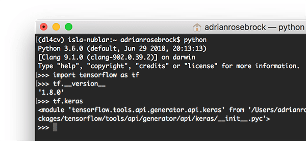
Figure 3: As you can see, by importing TensorFlow (as tf) and subsequently calling tf.keras, I’ve demonstrated in a Python shell that Keras is actually part of TensorFlow.

Including Keras inside tf.keras allows you to to take the following simple feedforward neural network using the standard Keras package:

# import the necessary packagesfrom keras.models import Sequentialfrom keras.layers.core import Denseimport tensorflow as tf # define the 3072-1024-512-3 architecture using Kerasmodel = Sequential()model.add(Dense(1024, input_shape=(3072,), activation=”sigmoid”))model.add(Dense(512, activation=”sigmoid”))model.add(Dense(10, activation=”softmax”))

from keras.models import Sequential

import tensorflow as tf

define the 3072-1024-512-3 architecture using Keras

model.add(Dense(1024, input_shape=(3072,), activation=”sigmoid”))

model.add(Dense(10, activation=”softmax”))

And then implement the same network using the tf.keras submodule which is part of TensorFlow:

# define the 3072-1024-512-3 architecture using tf.kerasmodel = tf.keras.models.Sequential()model.add(tf.keras.layers.Dense(1024, input_shape=(3072,), activation=”sigmoid”))model.add(tf.keras.layers.Dense(512, activation=”sigmoid”))model.add(tf.keras.layers.Dense(10, activation=”softmax”))

model = tf.keras.models.Sequential()

activation=”sigmoid”))

model.add(tf.keras.layers.Dense(10, activation=”softmax”))

Does this mean that you have to use tf.keras ? Is the standard Keras package now obsolete? No, of course not.

Keras as a library will still operate independently and separately from TensorFlow so there is a possibility that the two will diverge in the future; however, given that Google officially supports both Keras and TensorFlow, that divergence seems extremely unlikely.

The point is this:

If youâ€™re comfortable writing code using pure Keras, go for it, and keep doing it.

But if you find yourself working in TensorFlow, you should start leveraging the Keras API:

Itâ€™s built right into TensorFlow
Itâ€™s easier to use
And when you need pure TensorFlow to implement a specific feature or functionality, it can be dropped right into your Keras model.

There is no more Keras vs. TensorFlow argument — you get to have both and you get the best of both worlds.

Our example dataset

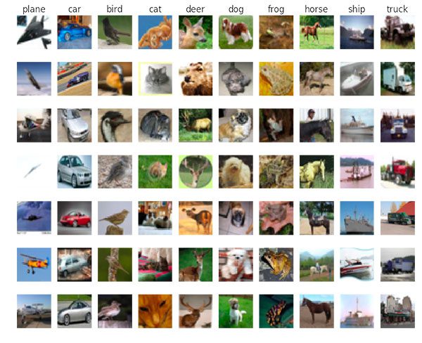
Figure 4: The CIFAR-10 dataset has 10 classes and is used for today’s demonstration (image credit).

For the sake of simplicity, we are going to be training two separate Convolutional Neural Networks (CNNs) on the CIFAR-10 dataset using:

Keras with a TensorFlow backend

The Keras submodule inside tf.keras

Iâ€™ll also be showing how to include custom TensorFlow code within your actual Keras model.

The CIFAR-10 dataset itself consists of 10 separate classes with 50,000 training images and 10,000 testing images. A sample is shown in Figure 4.

Our project structure

Our project structure today can be viewed in the terminal with the tree command:

$ tree –dirsfirst.â”œâ”€â”€ pyimagesearchâ”‚ â”œâ”€â”€ init.pyâ”‚ â”œâ”€â”€ minivggnetkeras.pyâ”‚ â””â”€â”€ minivggnettf.pyâ”œâ”€â”€ plot_keras.pngâ”œâ”€â”€ plot_tf.pngâ”œâ”€â”€ train_network_keras.pyâ””â”€â”€ train_network_tf.py 1 directory, 7 files

â”‚ â”œâ”€â”€ init.py

â”‚ â””â”€â”€ minivggnettf.py

â”œâ”€â”€ plot_tf.png

â””â”€â”€ train_network_tf.py

1 directory, 7 files

The pyimagesearch module is included with the downloads associated with this blog post. It is not pip-installable, but it is included in the “Downloads”. Let’s review the two important Python files part of the module:

minivggnetkeras.py : This is our strict Keras implementation of MiniVGGNet , a deep learning model based on VGGNet .

minivggnettf.py : This is our TensorFlow + Keras(i.e., tf.keras ) implementation of MiniVGGNet .

The root of the project folder contains two Python files:

train_network_keras.py : This is the first training script we’ll implement using strict Keras.

train_network_tf.py : The TensorFlow + Keras version of the training script is nearly identical; we’ll walk through it, highlighting differences, as well.

Each of the scripts will generate a respective training accuracy/loss plot as well:

plot_keras.png

plot_tf.png

As you can see from the directory structure, we’re going to be demonstrating the implementation + training of MiniVGGNet for both Keras and TensorFlow (with the tf.keras module) today.

Training a network with Keras

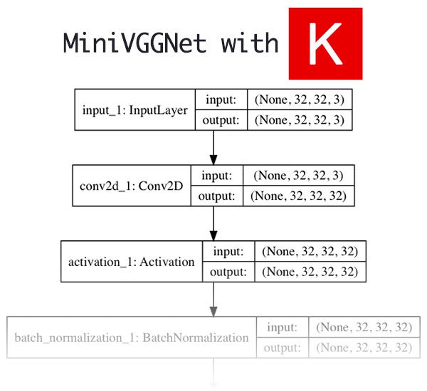
Figure 5: The MiniVGGNet CNN network architecture implemented using Keras.

The first step in training our network is to implement the network architecture itself in Keras.

Iâ€™ll assume you are already familiar with the fundamentals of training a neural network with Keras — if you are not, please refer to this introductory post.

Open up the minivggnetkeras.py file and insert the following code:

# import the necessary packagesfrom keras.layers.normalization import BatchNormalizationfrom keras.layers.convolutional import Conv2Dfrom keras.layers.convolutional import MaxPooling2Dfrom keras.layers.core import Activationfrom keras.layers.core import Dropoutfrom keras.layers.core import Densefrom keras.layers import Flattenfrom keras.layers import Inputfrom keras.models import Model

from keras.layers.normalization import BatchNormalization

from keras.layers.convolutional import MaxPooling2D

from keras.layers.core import Dropout

from keras.layers import Flatten

from keras.models import Model

We begin with a bunch of Keras imports required to build our model.

From there, we define our MiniVGGNetKeras class:

class MiniVGGNetKeras: @staticmethod def build(width, height, depth, classes): # initialize the input shape and channel dimension, assuming # TensorFlow/channels-last ordering inputShape = (height, width, depth) chanDim = -1 # define the model input inputs = Input(shape=inputShape)

@staticmethod

# initialize the input shape and channel dimension, assuming

inputShape = (height, width, depth)

inputs = Input(shape=inputShape)

We define the build method on Line 12, and define our inputShape and input . We’ll assume “channels last” ordering which is why depth is the last value in the inputShape tuple.

Let’s start defining the body of the Convolutional Neural Network:

23242526272829303132333435363738394041

# first (CONV => RELU) * 2 => POOL layer set x = Conv2D(32, (3, 3), padding=”same”)(inputs) x = Activation(“relu”)(x) x = BatchNormalization(axis=chanDim)(x) x = Conv2D(32, (3, 3), padding=”same”)(x) x = Activation(“relu”)(x) x = BatchNormalization(axis=chanDim)(x) x = MaxPooling2D(pool_size=(2, 2))(x) x = Dropout(0.25)(x) # second (CONV => RELU) * 2 => POOL layer set x = Conv2D(64, (3, 3), padding=”same”)(x) x = Activation(“relu”)(x) x = BatchNormalization(axis=chanDim)(x) x = Conv2D(64, (3, 3), padding=”same”)(x) x = Activation(“relu”)(x) x = BatchNormalization(axis=chanDim)(x) x = MaxPooling2D(pool_size=(2, 2))(x) x = Dropout(0.25)(x)

x = Conv2D(32, (3, 3), padding=”same”)(inputs)

x = BatchNormalization(axis=chanDim)(x)

x = Activation(“relu”)(x)

x = MaxPooling2D(pool_size=(2, 2))(x)

x = Conv2D(64, (3, 3), padding=”same”)(x)

x = BatchNormalization(axis=chanDim)(x)

x = Activation(“relu”)(x)

x = MaxPooling2D(pool_size=(2, 2))(x)

Examining the code block, you’ll notice we are stacking a series of convolutional, ReLU activation, and batch normalization layers prior to applying a pooling layer to reduce the spatial dimensions of the volume. Dropout is also applied to reduce overfitting.

For a brief review of the layer types and terminology, be sure to check out my previous Keras tutorial where they are explained. And for in-depth study, you should pick up a copy of my deep learning book, Deep Learning for Computer Vision with Python.

Let’s add the fully-connected (FC) layers to the network:

43444546474849505152535455565758

# first (and only) set of FC => RELU layers x = Flatten()(x) x = Dense(512)(x) x = Activation(“relu”)(x) x = BatchNormalization()(x) x = Dropout(0.5)(x) # softmax classifier x = Dense(classes)(x) x = Activation(“softmax”)(x) # create the model model = Model(inputs, x, name=”minivggnet_keras”) # return the constructed network architecture return model

x = Flatten()(x)

x = Activation(“relu”)(x)

x = Dropout(0.5)(x)

# softmax classifier

x = Activation(“softmax”)(x)

# create the model

return model

Our FC and Softmax classifier are appended onto the network. We then define the neural network model and return it to the calling function.

Now that weâ€™ve implemented our CNN in Keras, letâ€™s create the driver script that will be used to train it.

Open up train_network_keras.py and insert the following code:

12345678910111213141516171819

import matplotlib

from pyimagesearch.minivggnetkeras import MiniVGGNetKeras

from sklearn.metrics import classification_report

from keras.datasets import cifar10

import numpy as np

ap = argparse.ArgumentParser()

help=”path to output loss/accuracy plot”)

We import our required packages on Lines 2-13.

Notice the following:

On Line 3 the backend for Matplotlib is set to “Agg” so that we can save our training plots as image files. On Line 6 we import the MiniVGGNetKeras class. We’re using the scikit-learn’s LabelBinarizer for “one-hot” encoding and its classification_report to print classification accuracy statistics (Lines 7 and 8).

Our dataset is conveniently imported on Line 10. If you want to learn how to use custom datasets, I suggest you refer to this previous Keras tutorial or this post which shows how to a real-world of example with Keras.

Our only command line argument (our output –plot path) is parsed on Lines 16-19.

Let’s load CIFAR-10 and encode the labels:

21222324252627282930313233343536

# load the training and testing data, then scale it into the# range [0, 1]print(“[INFO] loading CIFAR-10 data…“)split = cifar10.load_data()((trainX, trainY), (testX, testY)) = splittrainX = trainX.astype(“float”) / 255.0testX = testX.astype(“float”) / 255.0 # convert the labels from integers to vectorslb = LabelBinarizer()trainY = lb.fit_transform(trainY)testY = lb.transform(testY) # initialize the label names for the CIFAR-10 datasetlabelNames = [“airplane”, “automobile”, “bird”, “cat”, “deer”, “dog”, “frog”, “horse”, “ship”, “truck”]

range [0, 1]

split = cifar10.load_data()

trainX = trainX.astype(“float”) / 255.0

lb = LabelBinarizer()

testY = lb.transform(testY)

initialize the label names for the CIFAR-10 dataset

“dog”, “frog”, “horse”, “ship”, “truck”]

We load and extract our training and testing splits on Lines 24 and 25) as well as convert to floating point + scale the data on Lines 26 and 27.

We encode our labels and initialize the actual labelNames on Lines 30-36.

Next, let’s train the model:

383940414243444546474849505152535455

train for, and batch size

EPOCHS = 30

print(“[INFO] compiling model…”)

model = MiniVGGNetKeras.build(width=32, height=32, depth=3,

model.compile(loss=”categorical_crossentropy”, optimizer=opt,

print(“[INFO] training network for {} epochs…“.format(EPOCHS))

batch_size=BS, epochs=EPOCHS, verbose=1)

The training parameters and optimization method are set (Lines 40-46).

Then we use our MiniVGGNetKeras.build method to initialize our model and compile it (Lines 47-50).

And subsequently, we kick off the training procedure (Lines 54 and 55).

Let’s evaluate the network and generate a plot:

575859606162636465666768697071727374

# evaluate the networkprint(“[INFO] evaluating network…“)predictions = model.predict(testX, batch_size=32)print(classification_report(testY.argmax(axis=1), predictions.argmax(axis=1), target_names=labelNames)) # plot the training loss and accuracyplt.style.use(“ggplot”)plt.figure()plt.plot(np.arange(0, EPOCHS), H.history[“loss”], label=”train_loss”)plt.plot(np.arange(0, EPOCHS), H.history[“val_loss”], label=”val_loss”)plt.plot(np.arange(0, EPOCHS), H.history[“acc”], label=”train_acc”)plt.plot(np.arange(0, EPOCHS), H.history[“val_acc”], label=”val_acc”)plt.title(“Training Loss and Accuracy on Dataset”)plt.xlabel(“Epoch #”)plt.ylabel(“Loss/Accuracy”)plt.legend(loc=”lower left”)plt.savefig(args[“plot”])

print(“[INFO] evaluating network…”)

print(classification_report(testY.argmax(axis=1),

plt.style.use(“ggplot”)

plt.plot(np.arange(0, EPOCHS), H.history[“loss”], label=”train_loss”)

plt.plot(np.arange(0, EPOCHS), H.history[“acc”], label=”train_acc”)

plt.title(“Training Loss and Accuracy on Dataset”)

plt.ylabel(“Loss/Accuracy”)

plt.savefig(args[“plot”])

Here we evaluate the network on our testing split of the data and generate a classification_report . Finally, we assemble and export our plot.

Note: Usually, I would serialize and export our model here so that it can be put to use in an image or video processing script, but we aren’t going to do that today as that is outside the scope of the tutorial.

To run our script, make sure you use the â€œDownloadsâ€� section of the blog post to download the source code.

From there, open up a terminal and execute the following command:

12345678910111213141516171819202122232425262728293031323334

$ python train_network_keras.pyUsing TensorFlow backend.[INFO] loading CIFAR-10 data…[INFO] compiling model…[INFO] training network for 30 epochs…Train on 50000 samples, validate on 10000 samplesEpoch 1/3050000/50000 [==============================] - 328s 7ms/step - loss: 1.7652 - acc: 0.4183 - val_loss: 1.2965 - val_acc: 0.5326Epoch 2/3050000/50000 [==============================] - 325s 6ms/step - loss: 1.2549 - acc: 0.5524 - val_loss: 1.1068 - val_acc: 0.6036Epoch 3/3050000/50000 [==============================] - 324s 6ms/step - loss: 1.1191 - acc: 0.6030 - val_loss: 0.9818 - val_acc: 0.6509…Epoch 28/3050000/50000 [==============================] - 337s 7ms/step - loss: 0.7673 - acc: 0.7315 - val_loss: 0.7307 - val_acc: 0.7422Epoch 29/3050000/50000 [==============================] - 330s 7ms/step - loss: 0.7594 - acc: 0.7346 - val_loss: 0.7284 - val_acc: 0.7447Epoch 30/3050000/50000 [==============================] - 324s 6ms/step - loss: 0.7568 - acc: 0.7359 - val_loss: 0.7244 - val_acc: 0.7432[INFO] evaluating network… precision recall f1-score support airplane 0.81 0.73 0.77 1000 automobile 0.92 0.80 0.85 1000 bird 0.68 0.56 0.61 1000 cat 0.56 0.55 0.56 1000 deer 0.64 0.77 0.70 1000 dog 0.69 0.64 0.66 1000 frog 0.72 0.88 0.79 1000 horse 0.88 0.72 0.79 1000 ship 0.80 0.90 0.85 1000 truck 0.78 0.89 0.83 1000 avg / total 0.75 0.74 0.74 10000

Using TensorFlow backend.

[INFO] compiling model…

Train on 50000 samples, validate on 10000 samples

50000/50000 [==============================] - 328s 7ms/step - loss: 1.7652 - acc: 0.4183 - val_loss: 1.2965 - val_acc: 0.5326

50000/50000 [==============================] - 325s 6ms/step - loss: 1.2549 - acc: 0.5524 - val_loss: 1.1068 - val_acc: 0.6036

50000/50000 [==============================] - 324s 6ms/step - loss: 1.1191 - acc: 0.6030 - val_loss: 0.9818 - val_acc: 0.6509

Epoch 28/30

Epoch 29/30

Epoch 30/30

[INFO] evaluating network…

automobile 0.92 0.80 0.85 1000

cat 0.56 0.55 0.56 1000

dog 0.69 0.64 0.66 1000

horse 0.88 0.72 0.79 1000

truck 0.78 0.89 0.83 1000

avg / total 0.75 0.74 0.74 10000

Each epoch is taking a little over 5 minutes to complete on my CPU.

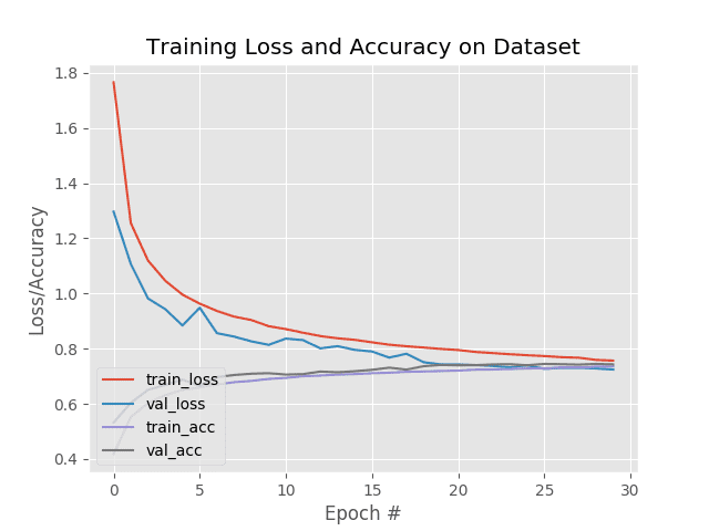
Figure 6: The accuracy/loss training curves are plotted with Matplotlib. This network was trained with Keras.

As we can see from the terminal output, we are obtaining 75% accuracy on our testing set — certainly not state-of-the-art; however, itâ€™s far better than random guessing (1/10).

For a small network, our accuracy is actually quite good!

And as our output plot demonstrates in Figure 6, there is no overfitting occurring.

Training a network with TensorFlow and `tf.keras`

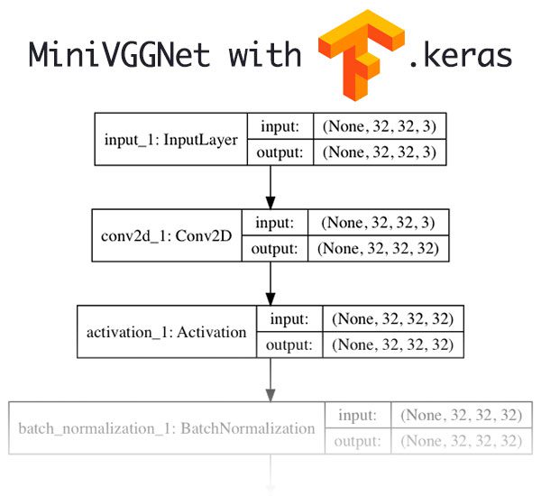
Figure 7: The MiniVGGNet CNN architecture built with tf.keras (a module which is built into TensorFlow) is identical to the model that we built with Keras directly. They are one and the same with the exception of the activation function which I have changed for demonstration purposes.

Now that weâ€™ve implemented and trained a simple CNN using the Keras library, letâ€™s learn how we can:

Implement the same network architecture using TensorFlowâ€™s tf.keras

Include a TensorFlow activation function inside our Keras model that is not implemented in Keras itself.

To get started, open up the minivggnettf.py file and weâ€™ll implement our TensorFlow version of MiniVGGNet :

1234567891011121314151617181920212223242526272829303132333435363738394041424344454647484950

# import the necessary packagesimport tensorflow as tf class MiniVGGNetTF: @staticmethod def build(width, height, depth, classes): # initialize the input shape and channel dimension, assuming # TensorFlow/channels-last ordering inputShape = (height, width, depth) chanDim = -1 # define the model input inputs = tf.keras.layers.Input(shape=inputShape) # first (CONV => RELU) * 2 => POOL layer set x = tf.keras.layers.Conv2D(32, (3, 3), padding=”same”)(inputs) x = tf.keras.layers.Activation(“relu”)(x) x = tf.keras.layers.BatchNormalization(axis=chanDim)(x) x = tf.keras.layers.Conv2D(32, (3, 3), padding=”same”)(x) x = tf.keras.layers.Lambda(lambda t: tf.nn.crelu(x))(x) x = tf.keras.layers.BatchNormalization(axis=chanDim)(x) x = tf.keras.layers.MaxPooling2D(pool_size=(2, 2))(x) x = tf.keras.layers.Dropout(0.25)(x) # second (CONV => RELU) * 2 => POOL layer set x = tf.keras.layers.Conv2D(64, (3, 3), padding=”same”)(x) x = tf.keras.layers.Lambda(lambda t: tf.nn.crelu(x))(x) x = tf.keras.layers.BatchNormalization(axis=chanDim)(x) x = tf.keras.layers.Conv2D(64, (3, 3), padding=”same”)(x) x = tf.keras.layers.Lambda(lambda t: tf.nn.crelu(x))(x) x = tf.keras.layers.BatchNormalization(axis=chanDim)(x) x = tf.keras.layers.MaxPooling2D(pool_size=(2, 2))(x) x = tf.keras.layers.Dropout(0.25)(x) # first (and only) set of FC => RELU layers x = tf.keras.layers.Flatten()(x) x = tf.keras.layers.Dense(512)(x) x = tf.keras.layers.Lambda(lambda t: tf.nn.crelu(x))(x) x = tf.keras.layers.BatchNormalization()(x) x = tf.keras.layers.Dropout(0.5)(x) # softmax classifier x = tf.keras.layers.Dense(classes)(x) x = tf.keras.layers.Activation(“softmax”)(x) # create the model model = tf.keras.models.Model(inputs, x, name=”minivggnet_tf”) # return the constructed network architecture return model

import tensorflow as tf

class MiniVGGNetTF:

def build(width, height, depth, classes):

# TensorFlow/channels-last ordering

chanDim = -1

# define the model input

x = tf.keras.layers.Conv2D(32, (3, 3), padding=”same”)(inputs)

x = tf.keras.layers.BatchNormalization(axis=chanDim)(x)

x = tf.keras.layers.Lambda(lambda t: tf.nn.crelu(x))(x)

x = tf.keras.layers.MaxPooling2D(pool_size=(2, 2))(x)

x = tf.keras.layers.Conv2D(64, (3, 3), padding=”same”)(x)

x = tf.keras.layers.BatchNormalization(axis=chanDim)(x)

x = tf.keras.layers.Lambda(lambda t: tf.nn.crelu(x))(x)

x = tf.keras.layers.MaxPooling2D(pool_size=(2, 2))(x)

x = tf.keras.layers.Flatten()(x)

x = tf.keras.layers.Lambda(lambda t: tf.nn.crelu(x))(x)

x = tf.keras.layers.Dropout(0.5)(x)

# softmax classifier

x = tf.keras.layers.Activation(“softmax”)(x)

# create the model

return model

In this file, notice that the imports are replaced by a single line (Line 2). The tf.keras sub-module contains all of our Keras functionality which we can call directly.

I’d like to call attention to the Lambda layers — they are used to insert a custom activation function, CRELU (Concatenated ReLUs), based on the paper Understanding and Improving Convolutional Neural Networks via Concatenated Rectified Linear Units by Shang et al. These lines are highlighted in yellow.

CRELUs are not implemented in Keras but are in TensorFlow — by using TensorFlow and tf.keras we can add CRELUs into our Keras model with just a single line of code.

Note: The CRELU has two outputs, one positiveReLU and one negative ReLU concatenated together. For positive x values the CRELU will return [x, 0] while for negative x values CRELU will return [0, x]. For more information, please refer to the Shang et al. publication.

The next step is to implement our TensorFlow + Keras driver script to train MiniVGGNetTF .

Open up train_network_tf.py and insert the following code:

1234567891011121314151617181920212223242526272829303132333435

# set the matplotlib backend so figures can be saved in the backgroundimport matplotlibmatplotlib.use(“Agg”) # import the necessary packagesfrom pyimagesearch.minivggnettf import MiniVGGNetTFfrom sklearn.preprocessing import LabelBinarizerfrom sklearn.metrics import classification_reportimport matplotlib.pyplot as pltimport tensorflow as tfimport numpy as npimport argparse # construct the argument parser and parse the argumentsap = argparse.ArgumentParser()ap.add_argument(“-p”, “–plot”, type=str, default=”plot_tf.png”, help=”path to output loss/accuracy plot”)args = vars(ap.parse_args()) # load the training and testing data, then scale it into the# range [0, 1]print(“[INFO] loading CIFAR-10 data…“)split = tf.keras.datasets.cifar10.load_data()((trainX, trainY), (testX, testY)) = splittrainX = trainX.astype(“float”) / 255.0testX = testX.astype(“float”) / 255.0 # convert the labels from integers to vectorslb = LabelBinarizer()trainY = lb.fit_transform(trainY)testY = lb.transform(testY) # initialize the label names for the CIFAR-10 datasetlabelNames = [“airplane”, “automobile”, “bird”, “cat”, “deer”, “dog”, “frog”, “horse”, “ship”, “truck”]

import matplotlib

from pyimagesearch.minivggnettf import MiniVGGNetTF

from sklearn.metrics import classification_report

import tensorflow as tf

import argparse

construct the argument parser and parse the arguments

ap.add_argument(“-p”, “–plot”, type=str, default=”plot_tf.png”,

args = vars(ap.parse_args())

load the training and testing data, then scale it into the

print(“[INFO] loading CIFAR-10 data…”)

((trainX, trainY), (testX, testY)) = split

testX = testX.astype(“float”) / 255.0

convert the labels from integers to vectors

trainY = lb.fit_transform(trainY)

labelNames = [“airplane”, “automobile”, “bird”, “cat”, “deer”,

Our imports are handled on Lines 2-12. The only changes in comparison to our Keras training script include importing the MiniVGGNetTF class and importing tensorflow as tf rather than Keras.

Our command line argument is parsed on Lines 15-18.

Then we load our data on Line 23 much like before.

The rest of the lines are the same — extracting training/testing splits and encoding our labels.

Let’s train our model:

37383940414243444546474849505152535455565758596061626364656667686970717273

# initialize the initial learning rate, total number of epochs to# train for, and batch sizeINIT_LR = 0.01EPOCHS = 30BS = 32 # initialize the optimizer and modelprint(“[INFO] compiling model…“)opt = tf.keras.optimizers.SGD(lr=INIT_LR, decay=INIT_LR / EPOCHS)model = MiniVGGNetTF.build(width=32, height=32, depth=3, classes=len(labelNames))model.compile(loss=”categorical_crossentropy”, optimizer=opt, metrics=[“accuracy”]) # train the networkprint(“[INFO] training network for {} epochs…“.format(EPOCHS))H = model.fit(trainX, trainY, validation_data=(testX, testY), batch_size=BS, epochs=EPOCHS, verbose=1) # evaluate the networkprint(“[INFO] evaluating network…“)predictions = model.predict(testX, batch_size=32)print(classification_report(testY.argmax(axis=1), predictions.argmax(axis=1), target_names=labelNames)) # plot the training loss and accuracyplt.style.use(“ggplot”)plt.figure()plt.plot(np.arange(0, EPOCHS), H.history[“loss”], label=”train_loss”)plt.plot(np.arange(0, EPOCHS), H.history[“val_loss”], label=”val_loss”)plt.plot(np.arange(0, EPOCHS), H.history[“acc”], label=”train_acc”)plt.plot(np.arange(0, EPOCHS), H.history[“val_acc”], label=”val_acc”)plt.title(“Training Loss and Accuracy on Dataset”)plt.xlabel(“Epoch #”)plt.ylabel(“Loss/Accuracy”)plt.legend(loc=”lower left”)plt.savefig(args[“plot”])

train for, and batch size

EPOCHS = 30

print(“[INFO] compiling model…”)

model = MiniVGGNetTF.build(width=32, height=32, depth=3,

model.compile(loss=”categorical_crossentropy”, optimizer=opt,

print(“[INFO] training network for {} epochs…“.format(EPOCHS))

batch_size=BS, epochs=EPOCHS, verbose=1)

evaluate the network

predictions = model.predict(testX, batch_size=32)

predictions.argmax(axis=1), target_names=labelNames))

plot the training loss and accuracy

plt.figure()

plt.plot(np.arange(0, EPOCHS), H.history[“val_loss”], label=”val_loss”)

plt.plot(np.arange(0, EPOCHS), H.history[“val_acc”], label=”val_acc”)

plt.xlabel(“Epoch #”)

plt.legend(loc=”lower left”)

The training process, taking place on Lines 39-54, is the same with the exception of those highlighted in yellow, where only minor changes are to be noted.

From there we evaluate and plot our data (Lines 58-73).

As you can see, we’ve implemented the exact same training process, only now weâ€™re using tf.keras .

To run this script, make sure you use â€œDownloadsâ€� section of the blog post to grab the code.

From there, open up a terminal and execute the following command:

123456789101112131415161718192021222324252627282930313233

$ python train_network_tf.py[INFO] loading CIFAR-10 data…[INFO] compiling model…[INFO] training network for 30 epochs…Train on 50000 samples, validate on 10000 samplesEpoch 1/3050000/50000 [==============================] - 457s 9ms/step - loss: 1.7024 - acc: 0.4369 - val_loss: 1.3181 - val_acc: 0.5253Epoch 2/3050000/50000 [==============================] - 441s 9ms/step - loss: 1.1981 - acc: 0.5761 - val_loss: 1.1025 - val_acc: 0.6072Epoch 3/3050000/50000 [==============================] - 441s 9ms/step - loss: 1.0506 - acc: 0.6317 - val_loss: 1.0647 - val_acc: 0.6227…Epoch 28/3050000/50000 [==============================] - 367s 7ms/step - loss: 0.6798 - acc: 0.7611 - val_loss: 0.7161 - val_acc: 0.7479Epoch 29/3050000/50000 [==============================] - 364s 7ms/step - loss: 0.6732 - acc: 0.7639 - val_loss: 0.6969 - val_acc: 0.7544Epoch 30/3050000/50000 [==============================] - 366s 7ms/step - loss: 0.6743 - acc: 0.7641 - val_loss: 0.6973 - val_acc: 0.7550[INFO] evaluating network… precision recall f1-score support airplane 0.86 0.69 0.76 1000 automobile 0.93 0.79 0.85 1000 bird 0.75 0.59 0.66 1000 cat 0.59 0.55 0.57 1000 deer 0.65 0.78 0.71 1000 dog 0.70 0.66 0.68 1000 frog 0.67 0.93 0.78 1000 horse 0.90 0.75 0.82 1000 ship 0.81 0.91 0.86 1000 truck 0.80 0.89 0.84 1000 avg / total 0.76 0.76 0.75 10000

[INFO] loading CIFAR-10 data…

[INFO] training network for 30 epochs…

Epoch 1/30

Epoch 2/30

Epoch 3/30

…

50000/50000 [==============================] - 367s 7ms/step - loss: 0.6798 - acc: 0.7611 - val_loss: 0.7161 - val_acc: 0.7479

50000/50000 [==============================] - 364s 7ms/step - loss: 0.6732 - acc: 0.7639 - val_loss: 0.6969 - val_acc: 0.7544

50000/50000 [==============================] - 366s 7ms/step - loss: 0.6743 - acc: 0.7641 - val_loss: 0.6973 - val_acc: 0.7550

precision recall f1-score support

airplane 0.86 0.69 0.76 1000

bird 0.75 0.59 0.66 1000

deer 0.65 0.78 0.71 1000

frog 0.67 0.93 0.78 1000

ship 0.81 0.91 0.86 1000

After training completes you have a training plot that look similar to the following:

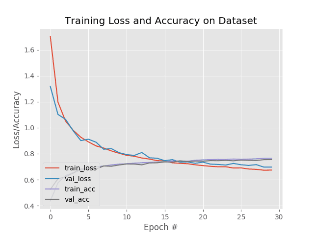
Figure 8: The deep learning training plot shows our accuracy and loss curves. The CNN was trained with the Keras module which is built into TensorFlow.

By swapping in the CRELU for the RELU activation function we obtain 76% accuracy; however, that 1% increase may be due to the random initialization of the weights in the network — further experiments with cross-validation would be required to demonstrate that CRELU was indeed responsible for this increase of accuracy.

However, the raw accuracy is not the important aspect of this section.

Instead, focus on how we were able to swap in a TensorFlow activation function in-place of a standard Keras activation function inside of a Keras model!

You could do the same with your own custom activation functions, loss/cost functions, or layer implementations as well.

Summary

In todayâ€™s blog post we discussed questions surrounding Keras vs. TensorFlow, including:

Should I be using Keras vs. TensorFlow for my project?
Is TensorFlow or Keras better?
Should I invest my time studying TensorFlow? Or Keras?

Ultimately, we found that trying to decide between Keras and TensorFlow is starting to become more and more irrelevant.

The Keras library has been integrated directly into TensorFlow via the tf.keras module.

Essentially, you can code your model and training procedures using the easy to use Keras API and then custom implementations into the model or training process using pure TensorFlow!

If youâ€™re spinning your wheels trying to just get started with deep learning, trying to decide between Keras or TensorFlow for your next project, or simply wondering if Keras or TensorFlow is â€œbetterâ€�…then itâ€™s time you seek some traction.

My advice to you is simple:

Just get started.

Type either import keras or import tensorflow as tf (so you have access to tf.keras ) into your Python project and get to work.

TensorFlow can be directly integrated into your model or training process so thereâ€™s no need to compare features, functionality, or ease of use — all of TensorFlow and Keras are available for you to use in your projects.

I hope you enjoyed todayâ€™s blog post!

If you are interested in getting started with computer vision and deep learning, I would suggest you take a look at my book, Deep Learning for Computer Vision with Python. Inside the book, I utilize Keras and TensorFlow to teach you deep learning applied to computer vision applications.

And if you would like to download the source code todayâ€™s tutorial (and be notified when future blog posts are published here on PyImageSearch), just enter your email address in the form below!

Keras vs. TensorFlow – Which one is better and which one should I learn?

Adrian Rosebrock

Keras vs. TensorFlow – Which one is better and which one should I learn?

If youâ€™re asking â€œKeras vs. TensorFlowâ€�, youâ€™re asking the wrong question

Keras is built into TensorFlow via the â€œtf.kerasâ€� module

define the 3072-1024-512-3 architecture using Keras

Our example dataset

Our project structure

Training a network with Keras

range [0, 1]

initialize the label names for the CIFAR-10 dataset

train for, and batch size

Training a network with TensorFlow and `tf.keras`

construct the argument parser and parse the arguments

load the training and testing data, then scale it into the

convert the labels from integers to vectors

train for, and batch size

evaluate the network

plot the training loss and accuracy

Summary

Downloads:

Keras vs. TensorFlow – Which one is better and which one should I learn?

If youâ€™re asking â€œKeras vs. TensorFlowâ€�, youâ€™re asking the wrong question

Keras is built into TensorFlow via the â€œtf.kerasâ€� module

define the 3072-1024-512-3 architecture using Keras

Our example dataset

Our project structure

Training a network with Keras

range [0, 1]

initialize the label names for the CIFAR-10 dataset

train for, and batch size

Training a network with TensorFlow and tf.keras

construct the argument parser and parse the arguments

load the training and testing data, then scale it into the

convert the labels from integers to vectors

train for, and batch size

evaluate the network

plot the training loss and accuracy

Summary

Downloads:

Training a network with TensorFlow and `tf.keras`