Previously, we’ve seen some of the very basic image analysis operations in Python. In this last part of basic image analysis, we’ll go through some of the following contents.
Following contents is the reflection of my completed academic image processing course in the previous term. So, I am not planning on putting anything into production sphere. Instead, the aim of this article is to try and realize the fundamentals of a few basic image processing techniques. For this reason, I am going to stick to using SciKit-Image - numpy mainly to perform most of the manipulations, although I will use other libraries now and then rather than using most wanted tools like OpenCV :
I wanted to complete this series into two section but due to fascinating contents and its various outcome, I have to split it into four parts. You can find the first three here:
| Part 1 | Part 2 | Part 3 |
Now, let’s get started!
Thresholding
Ostu’s Method
Thresholding is a very basic operation in image processing. Converting a greyscale image to monochrome is a common image processing task. And, a good algorithm always begins with a good basis!
Otsu thresholding is a simple yet effective global automatic thresholding method for binarizing grayscale images such as foregrounds and backgrounds. In image processing, Otsu’s thresholding method (1979) is used for automatic binarization level decision, based on the shape of the histogram. It is based entirely on computation performed on the histogram of an image.
The algorithm assumes that the image is composed of two basic classes: Foreground and Background. It then computes an optimal threshold value that minimizes the weighted within class variances of these two classes.
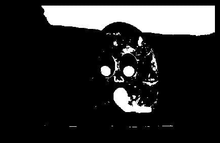
Otsu threshold is used in many applications from medical imaging to low-level computer vision. It’s many advantages and assumptions.
Mathematical Formulation of Otsu method. This will redirect you to my homepage where we explained mathematics behind Otsu method.
Algorithm
If we incorporate a little math into that simple step-wise algorithm, such an explanation evolves:
-
Compute histogram and probabilities of each intensity level.
-
Set up initial wiand μi.
Step through from threshold t = 0to t = L-1:
-
update: wi and μi
-
compute: σ2b(t)
The Desired threshold corresponds to the maximum value of σ2b(t).

Nice but not Great. Otsu’s method exhibits the relatively good performance if the histogram can be assumed to have bimodal distribution and assumed to possess a deep and sharp valley between two peaks.
So, now if the object area is small compared with the background area, the histogram no longer exhibits bimodality and if the variances of the object and the background intensities are large compared to the mean difference, or the image is severely corrupted by additive noise, the sharp valley of the gray level histogram is degraded.
As a result, the possibly incorrect threshold determined by Otsu’s method results in the segmentation error. But we can further improve Otsu’s method.
KMeans Clustering
k-means clustering is a method of vector quantization, originally from signal processing, that is popular for cluster analysis in data mining.
In Otsu thresholding, we found the threshold which minimized the intra-segment pixel variance. So, rather than looking for a threshold from a gray level image, we can look for clusters in color space, and by doing so we end up with the K-means clustering technique.
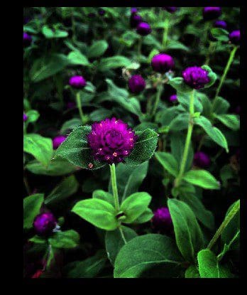
For clustering the image, we need to convert it into a two-dimensional array.
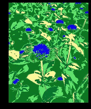
Next, we use scikit-learn’s cluster method to create clusters. We pass n_clustersas 5 to form five clusters. The clusters appear in the resulting image, dividing it into five parts with distinct colors.
The clustering number 5 was chosen heuristically for this demonstration. One can change the number of clusters to visually validate image with different colors and decide that closely matches the required number of clusters.
Once the clusters are formed, we can recreate the image with the cluster centers and labels to display the image with grouped patterns.
Line Detection
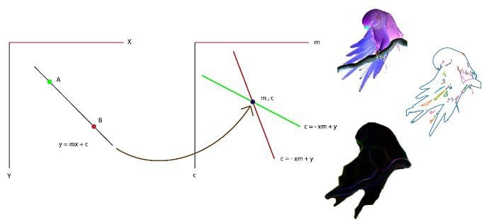
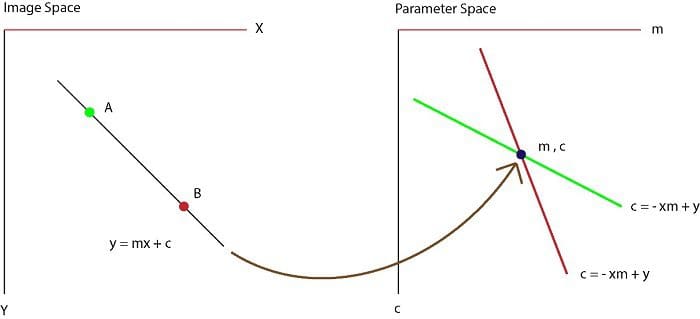
Hough TransformHough Transform is a popular technique to detect any shape if we can represent that shape in mathematical form. It can detect the shape even if it is broken or distorted a little bit. We won’t go too deeper to analyze the mechanism of Hough transform rather than giving intuitive mathematical description before implementing it on code and also provide some resource to understand it more in details.
Mathematical Formulation of Hough Transform. This will redirect you to my homepage where we explained mathematics behind Hough Transform method.
Algorithm
- Corner or edge detection
ρrange and θ range creation
-
ρ : -Dmax to Dmax
-
θ : -90 to 90
Hough accumulator
-
2D array with the number of rows equal to the number of ρvalues and the number of columns equal to the number of θ
-
For each edge point and for each θ value, find the nearest ρvalue and increment that index in the accumulator.
-
Local maxima in the accumulator indicate the parameters of the most prominent lines in the input image.
Edge Detection
Edge detection is an image processing technique for finding the boundaries of objects within images. It works by detecting discontinuities in brightness. Common edge detection algorithms include
-
Sobel
-
Canny
-
Prewitt
-
Roberts and
-
fuzzy logic methods.
Here, We’ll cover one of the most popular methods, which is the Canny Edge Detection.
Canny Edge Detection
A multi-stage edge detection operation capable of detecting a wide range of edges in images. Now, the Process of Canny edge detection algorithm can be broken down into 5 different steps:
-
Apply Gaussian Filter
-
Find the intensity gradients
-
Apply non-maximum suppression
-
Apply double threshold
-
Track edge by hysteresis.
Let’s understand each of them intuitively. For a more comprehensive overview, please check the given link at the end of this article. However, this article is already becoming too big, so we decide not to provide the full implementation of code here rather than giving an intuitive overview of an algorithm of that code. But one can skip and jump to the repo for the code :)
The process of Canny Edge Detection. . This will redirect you to my homepage where we explained mathematics behind Canny Edge method.
At that ends the 4-part series on Basic Image-Processing in Python. I hope everyone was able to follow along, and if you feel that I have done an important mistake, please let me know in the comments!
The entire source code is available on : GitHub.
Related: