“There’s the part you’ve braced yourself against, and then there’s the other part” – The Mountain Goats
My favourite genre of movie is Nicole Kidman in a questionable wig. (Part of the sub-genre founded by Sarah Paulson, who is the patron saint of obvious wigs.) And last night I was in the same room* as Nicole Kidman to watch a movie where I swear she’s wearing the same wig Dolly did in Steel Magnolias. All of which is to say that Boy Erased is an absolutely brilliant and you should all rush out to see it when it’s released. (There are many good things about it that aren’t Nicole Kidman’s wig.) You will probably cry.
When I eventually got home, I couldn’t stop thinking of one small moment towards the end of the film where one character makes a peace overture to another character that is rejected as being insufficient after all that has happened. And it very quietly breaks the first character’s heart. (Tragically this is followed by the only bit of the movie that felt over-written and over-acted, but you can’t have it all.)
So in the spirit of blowing straight past nuance and into the point that I want to make, here is another post about priors. The point that I want to make here is that saying that there is no prior information is often incorrect. This is especially the case when you’re dealing with things on the log-scale.
Collapsing Stars
Last week, Jonah an I successfully defended our visualization paper against a hoard of angry** men*** in Cardiff. As we were preparing our slides, I realized that we’d missed a great opportunity to properly communicate how bad the default priors that we used were.
 This figure (from our paper) plots one realization of fake data generated from our prior against the true data. As you can see, the fake data simulated from the prior model is two orders of magnitude too large.
(While plotting against actual data is a convenient way of visualizing just how bad these priors are, we could see the same information using a histogram.)
To understand just how bad these priors are, let’s pull in some physical comparisons. PM2.5 (airborne particulate matter that is less than 2.5 microns in diameter) is measured in micrograms per cubic metre. So let’s work out the density of some real-life things and see where they’d fall on the y-axis of that plot.
(And a quick note for people who are worried about talking the logarithm of a dimensioned quantity: Imagine I’ve divided through by a baseline of 1 microgram per cubic metre. To do this properly, I probably should divide through by a counterfactual, which would be more reasonably around 5 micrograms per cubic metre, but let’s keep this simple.)
Some quick googling gives the following factlets:
-
The log of the density of concrete would be around 28.
-
The log the density of a neutron star would be around 60.
Both of these numbers are too small to appear on the y-axis of the above graph. That means that every point in that prior simulation is orders of magnitude denser than the densest thing in the universe.
It makes me wonder why I would want to have any prior mass at all on these types of values. Sometimes, such as in the example in the paper, it doesn’t really matter. The data informs the parameters sufficiently well that the silly priors don’t have much of an effect on the inference.
But this is not always the case. In the real model for air pollution, that our model was the simplest possible version of, it’s possible that some of the parameters will be hard to learn from data. In this case, these un-phyiscal priors will lead to unphysical inference. (In particular, the upper end of the credible interval on the posterior predictive interval will be unreasonable.)
The nice thing here is that we don’t really need to know anything about air pollution to make weakly informative priors that are tailored for this data. All we need to know is that if you breathe try to breathe in concrete, you will die. This means that we just need to set priors that don’t generate values that are bigger than 28. I’ve talked about this idea of containment priors in these pages before, but a concrete example hopefully makes it more understandable. (That pun is unforgivable and I love it!)
The Recognition Scene
The nice thing about this example is that it is readily generalizable to a lot of cases where logarithms are used.
In the above case, we modelled log-PM2.5 for two reasons: because it was more normal, but more importantly because we care much more about the difference between 


A different time you see logarithms is when you’re modelling count data. Once again, there are natural limits to how big counts can be.
Firstly, it is always good practice to model relative-risk rather than risk. That is to say that if we observe 


rather than

The reason for doing this is that if the expected number of counts differs strongly between observations, the relative risk 

This is relevant for setting priors on model parameters. If we follow usual practice and model 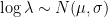

But that assumes that our transformation of our counts to unit scale was reasonable. We can do more than that!
Because we do inference using computers, we are limited to numbers that computers can actually store. In particular, we know that if 
This strongly suggests that if the covariates used in 
Once again, this is the most extreme priors for a *generic *Poisson model that don’t put too much weight on completely unreasonable values. Some problem-specific though can usually make these priors even tighter. For instance, we know there are fewer than seven and a half billion people on earth, so anything that is counting people can safely use much tighter priors (in particular we don’t want too much mass on sigma that’s bigger than 7).
All of these numbers are assuming that 
The exact same arguments can be used to put priors on the hyper-parameters in models of count data (such as models that use a negative-binomial likelihood). Similarly, priors for models of positive, continuous data can be set using the sorts of arguments used in the previous section.
Song For an Old Friend
This really is just an extension of the type of thing that Andrew has been saying for years about sensible priors for the logit-mean in multilevel logistic regression models. In that case, you want the priors for the logit-mean to be contained within [-5,5].
The difference between this case and they types of models considered in this post, is that the upper bound requires some more information than just the structure of the likelihood. In the first case, we needed information about the real world (concrete, neutron stars etc), while for count data we needed to know about the limits of computers.
But all of this information is easily accessible. All you have to do is remember that you’re probably not as ignorant as you think you are.
Just to conclude, I want to remind everyone once again that there is one true thing that we must always keep in mind when specifying priors. When you specify a prior, just like when you cut a wig, you need to be careful. That hair isn’t going to grow back.
Deserters
* It was a very large room. I had to zoom all the way in to get a photo of her. It did not come out well.)
** They weren’t.
*** They were. For these sort of sessions, the RSS couldn’t really control who presented the papers (all men) but they could control the chair (a man) and the invited discussants (both men). But I’m sure they asked women and they all said no. </sarcasm> Later, two women contributed very good discussions from the floor, so it wasn’t a complete sausage-fest.