Logistic Regression： Concept & Application

Through this article, we try to understand the concept of the logistic regression and its application. We will, as usual, deep dive into the model building in R and look at ways of validating our logistic regression model and more importantly understand it rather than just predicting some values.We will be covering1. Categorical and numerical variables2. Why linear regression is not fit for classification3. Understanding how logistic regression works4. Assumptions of logistic regression5. Building logistic regression model in R6. Measuring performance of model using confusion matrix and ROC curve7. Improving performance of the logistic model

In my previous article on multiple linear regression, we predicted the cab price I will be paying in the next month. Here the final cab price, which we were predicting, is a numerical variable. In very simple terms, it was a number which varied over a range of values. But now there is one more data type which we should first understand before diving into logistic regression.

Types of data

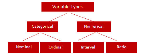
• Categorical: Categorical variables take on values that are names or labels. The color of a ball (e.g., red, green, blue) or the breed of a dog (e.g., collie, shepherd, terrier) would be examples of categorical variables.

• Quantitative: Quantitative variables are numerical. They represent a measurable quantity. For example, when we speak of the population of a city, we are talking about the number of people in the city — a measurable attribute of the city. Therefore the population would be a quantitative variable.

Categorical

• Nominal: Nominal values are the type of categorical variables that represent a discrete category which does not contain any kind of order within them. For example, say male and female are nominal categorical values because they are discrete and they do not have any implied order. Suppose we represent all males by 1 and all females by 0, then we can not imply that 1 is greater than 0 or vice-versa

• Ordinal: Ordinal values are the type of categorical variables that represent again a discrete category but they do have an implied order within them. For instance, let us take the speed of a fan which can be stated say low, medium and high. If we denote low by 0, medium by 1 and high by 2 then we can still imply that 1>0 since the medium speed of the fan is greater than the low speed of the fan. Here there is an implicit order in discrete values.

There is another class of machine learning problems which involve predicting a categorical variable rather than predicting a variable which is continuous in nature. These type of machine learning problems where our aim is to predict a categorical variable are known as classification problems.

So in very simple terms, classification is about predicting a label and regression is about predicting a quantity.

Logistic regression is a method for fitting a regression curve, y = f(x) when y is a categorical variable. It is a classification algorithm used to predict a binary outcome (1 / 0, Yes / No, True / False) given a set of independent variables.

A logistic regression model can be represented by the equation

• p is the probability of an event to happen which you are trying to predict

• x1, x2 and x3 are the independent variables which determine the occurrence of an event i.e. p

• a0 is the constant term which will be the probability of the event happening when no other factors are considered

• R.H.S represent the link function which will help us to determine a non-linear relation in a linear way wherein (p/1-p) is the odd ratio. Whenever the log of the odds ratio is found to be positive, the probability of success is always more than 50%.

Before going any further let us quickly see why we can not use linear regression for a classification problem and how logistic regression comes to our rescue there

Let us take a small case here, suppose we have a model whose only job is to look at the fruit in front of the camera and state whether it is an apple or not. This is a simple binary classification problem where our output variable can take only 2 states(yes/no or 0/1). Our model gives an output 1 if it recognises it as an apple and output 0 if it is not an apple.

Let us build a simple linear regression model for this classification case and see why it is not a good idea to solve a classification problem using linear regression.

Now it is time to visualize our linear regression model here ….

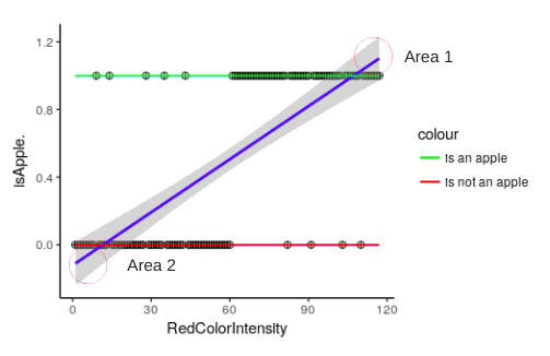
• 1 represents all the points which are classified as an apple
• 0 represents all the points which are not apple
• The line in blue is a “best fit” line plotted by our linear regression model

Issue 1: Area 1 and Area 2 represent a portion of the line where the probability of any fruit seen by our model being an apple is >1(area1) and <0(area2). Since probabilities can never be greater than 1 or less than 0, part of the regression line in area 1 and area 2 does not make any sense.

Solution 1: Since both, the areas are not required, we cut them and keep the remaining with us. This line has a finite limit. Whenever your x tends to infinity, y will tend to 1 and whenever your x will tend to -infinity, y will tend to 0.

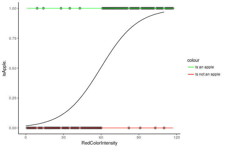
Issue 2: Since binary classification problems can only have one of two possible values(0 or 1), the residuals(Actual value -predicted value) will not be normally distributed about the regression line.

Solution 2: To overcome the residual issue, we identify a threshold probability value. Our final variable in logistic regression is the probability of the target event. So if my apple identifier logistic model outputs a value like 0.45 then this means that there is a 45% probability that new fruit seen by our model is an apple. Here we set a threshold value 0.5 which means that if the probability of fruit seen by the model is an apple is greater than 50% then our model will predict it to be an apple and if it is less than 50% then our model will say that it is not an apple.

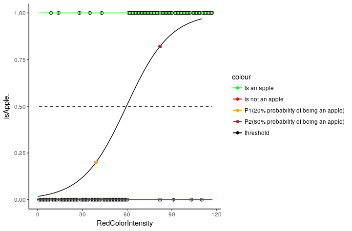
So every value predicted by the model below 0.5, the model will classify it as not an apple in this case and for every other value greater than threshold 0.5, the model will classify it as an apple.

Assumptions in logistic regression

There are some assumptions which need to be satisfied for having a logistic regression model which we can interpret meaningfully.

But let us look at some things which we no longer have to take care of in the case of logistic regression if we compare it with logistic regression.

• Logistic regression does NOT require a linear relationship between the dependent and independent variables

• The error terms (residuals) do NOT need to be normally distributed

• Homoscedasticity is NOT required

• The dependent variable in logistic regression is NOT measured on an interval or ratio scale

But then there are some assumptions which should hold

• Logistic regression requires the dependent variable to be categorical

• Logistic regression requires there to be little or no multicollinearity among the independent variables. This means that the independent variables should not be too highly correlated with each other.

• There should be a linear relationship between the link function (log(p/(1-p))and independent variables in the logit model.

Problem Statement: The diabetes dataset consists of several medical predictor variables and one target variable, Outcome. Predictor variables include the number of pregnancies the patient has had, their BMI, insulin level, age, and so on. The objective is to diagnostically predict whether or not a patient has diabetes, based on certain diagnostic measurements included in the dataset.

Loading dataset

There are 9 columns in our dataset which includes 8 predictor variables (Pregnancies, Glucose, Blood Pressure .. etc) and 1 target variable (Outcome). The patients diagnosed with diabetes are represented 1 and patients which were not diagnosed with diabetes are represented with 0.

Building a logistic regression model

Let us straight away build a simplest logistic regression model using the glm function in R. The glm function expects the first parameter as the target variable (Outcome) and then predictor variables after “~” sign.A “dot” in the place of predictor variables signify that all the columns in the dataset (obviously apart from target variable) are taken into the consideration to predict the target variable (Outcome). data parameter takes the training data as input and family in glm should be set to binomial in this case.

Why family = binomial?

We set the family parameter to binomial because the variable to predict (Outcome) is binary(0/1), however, logistic regression can also be used to predict a dependent variable which can assume more than 2 values. In this second case, we call the model “multinomial logistic regression”. A typical example, for instance, would be classifying films between “Entertaining”, “borderline” or “boring”.

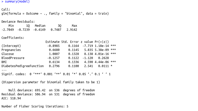
Let us have a closer look at what all the above terms are in the summary of our logistic model which will help us to gain a better understanding of the model we have built.

• Null Deviance: When the model includes only an intercept term (no predictor variables are taken into account), then the performance of the model is governed by null deviance.

• Residual Deviance: When the model has included 6 predictor variables, then the deviance is residual deviance which is lower(506.94) than null deviance(695.42). The lower value of residual deviance points out that the model has become better when it has included predictor variables

• AIC value: Its full form is Akaike Information Criterion (AIC). This is useful when we have more than one model to compare the goodness of fit of the models. It is a maximum likelihood estimate which penalizes to prevent overfitting. It measures the flexibility of the models. It is analogous to adjusted R squared in multiple linear regression where it tries to prevent you from including irrelevant predictor variables. Lower AIC of a model is better than the model having higher AIC.

• Fisher score: It tells how the model was estimated. The algorithm looks around to see if the fit would be improved by using different estimates. If it improves then it moves in that direction and then fits the model again. The algorithm stops when no significant additional improvement can be done. “Number of Fisher Scoring iterations,” tells “how many iterations this algorithm run before it stopped”.Here it is 5.

Predicting whether the new person coming for diagnosis will be diabetic or not

Now we’ll perform a quick evaluation on the test set by plotting the probability (score) estimated by our model with a double density plot.

Given that our model’s final objective is to classify new instances into one of two categories, whether the patient is having diabetes or not we will want the model to give high scores to positive instances ( 1: patients with diabetes) and low scores (0: patients without diabetes ) otherwise. Thus for an ideal double density plot, you want the distribution of scores to be separated, with the score of the negative instances to be on the left and the score of the positive instance to be on the right.

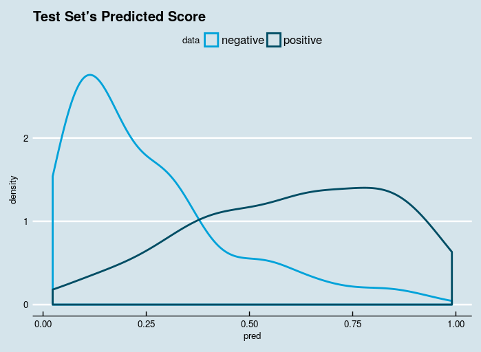
Since the separation between negative points and positive data points is well enough, hence we can proceed forward with this model.

Setting threshold and classifying the predicted probabilities to 0 or 1

In the predict function, we passed our logistic regression model as an input to the first parameter and setting type as “response”. In new data parameter, we passed our test set without the target (Outcome) column.

Then in the second line, we set the threshold value to 0.5. As we already discussed,

• Any probability value predicted by our logistic regression model which will be less than the threshold will be converted to 0

• Any probability value predicted by our logistic regression model which will be greater than the threshold will be converted to 1

Then we make a data frame to view original outcome and the outcome predicted by our model.

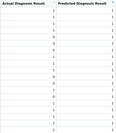
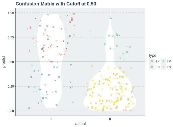
Our model was able to predict correctly for many patients coming in that which ones will have diabetes but there were some patients for which our model predicted that they have diabetes although they were not actually diabetic.

Measuring the performance of our logistic regression model

1. Confusion Matrix

A confusion matrix is a table that is often used to describe the performance of a classification model (or “classifier”) on a set of test data for which the true values are known.

Let us directly create a confusion matrix for our logistic regression model and understand it in the process

Understanding from the matrix

• There are two possible outcomes for prediction i.e. either a yes or a no. Yes means that the given patient will be diagnosed with diabetes and no means the patient will not be diagnosed with diabetes.

• Classifier made a total of 231 (121+13+43+54) predictions for the diagnosed patients

• Out of cases, our model predicted YES 67 (13+54) times and “NO” only 164 (121+43) times

• In reality, 134 (121+13) patients were not diagnosed with diabetes and 97 (43+54) patients were diagnosed with diabetes.

Key terms in confusion matrix

• True Positive (TP): This refers to the cases in which we predicted “YES” and our prediction was actually TRUE(Patient is actually having diabetes)

• True Negative(TN): This refers to the cases in which we predicted “NO” and our prediction was actually TRUE(Patient was not having diabetes)

• False Positive(FP): This refers to the cases in which we predicted “YES”, but our prediction turned out FALSE(Patient was not having diabetes but our model predicted that he is diabetic)

• False Negative(FN): This refers to the cases in which we predicted “NO” but our prediction turned out FALSE(Patient was diabetic but our model predicted that he is not having diabetes)

Understanding model performance metrics in classification problems

The accuracy of the model is not the only criteria to measure the performance of a classification model

• Accuracy: Overall, how often is the classifier correct?( TP + TN )/TOTAL = ( 121+54 )/231 = 0.757

• Misclassification Rate: Overall, how often is it wrong?1-Accuracy = 0.243

• True Positive Rate: When it’s actually yes, how often does it predict yes?TP/Actual Yes = 54/(43+54) = 0.5596

• False Positive Rate: When it’s actually no, how often does it predict yes?FP/Actual No = 13/(121+13) = 0.08441

• Specificity: When it’s actually no, how often does it predict no?TN/Actual No = 121/(121+13)= 0.9156

• Precision: When it predicts yes, how often is it correct?TP/Predicted Yes = 54/(54+13) = 0.8059

• Prevalence: How often does the yes condition actually occur in our sample?Actual Yes/Total = (43+54)/231 = 0.4199

2. ROC Curve

1. Senstivity and specificity trade off

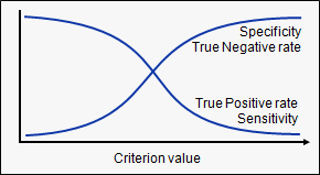
• Most machine learning classifiers produce real-valued scores that correspond with the strength of the prediction that a given case is positive. Turning these real-valued scores into yes or no predictions require setting a threshold; cases with scores above the threshold are classified as positive, and cases with scores below the threshold are predicted to be negative.
• Different threshold values give different levels of sensitivity and specificity.
• A high threshold is more conservative about labeling a case as positive; this makes it less likely to produce false positive results but more likely to miss cases that are in fact positive (lower rate of true positives).A low threshold produces positive labels more liberally, so it is less specific (more false positives) but also more sensitive (more true positives).

2. What are ROC curves

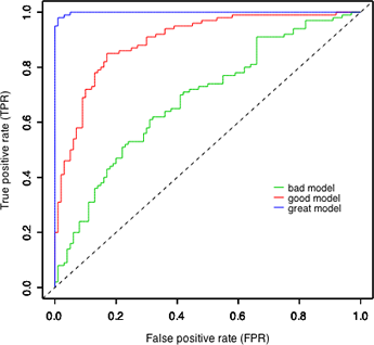
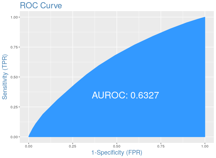
ROC curves are commonly used to characterize the sensitivity/specificity tradeoffs for a binary classifier. The ROC curve plots true positive rate against false positive rate, giving a picture of the whole spectrum of such trade-offs.

3. What is AUROC ( Area under ROC )

The accuracy of the test depends on how well the model separates the group into two classes(in the case of binary classification). Accuracy is measured by the area under the ROC curve. An area of 1 represents a perfect test; an area of .5 represents a worthless test. A rough guide for classifying the accuracy of a test is the traditional academic point system:

• .90–1 = excellent (A)

• .80-.90 = good (B)

• .70-.80 = fair ©

• .60-.70 = poor (D)

• .50-.60 = fail (F)

4. Why is ROC a good metric

• The ROC is invariant against class skew of the applied data set — that means a data set featuring 60% positive labels will yield the same (statistically expected) ROC as a data set featuring 45% positive labels (though this will affect the cost associated with a given point of the ROC). Hence it is capable of handling imbalance in the data set as it not dependent on it in any way

• The ROC is invariant against the evaluated score — which means that we could compare a model giving non-calibrated scores like a regular linear regression with a logistic regression or a random forest model whose scores can be considered as class probabilities.

Getting optimal threshold value

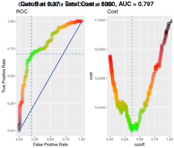
Since the prediction of a logistic regression model is a probability, in order to use it as a classifier, we’ll have to choose a cutoff value, or you can say it a threshold value. Where scores above this value will be classified as positive, those below as negative. By default, we take threshold at 0.5.

We then try to find an optimal threshold value for our case.

Cuttoff plot code

Assigning false positive cases a penalty value

cost_false_positisve <- 100

Assigning false negative cases a penalty value

cost_false_negative <- 200 ##Plotting ROC and Cost curve roc_info <- ROCInfo( data = cm_info$data, predict = “predict”, actual = “actual”, cost.fp = cost_false_positve, cost.fn = cost_false_negative ) grid.draw(roc_info$plot) Cut off point at 0.37 is the point where we have the lowest associated cost and the maximum area we can cover with this lowest cost.

Let us set the threshold to 0.37 and try to visualize results again

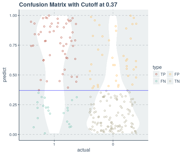
With this process, we were able to improve the performance of our logistic model. We can further improve the performance of the model by selecting only the important variables and then building the model as I did in my previous article on multiple regression.

this article, I tried to cover the basic idea of a classification problem by trying to solve one using logistic regression. We also understood how to evaluate a model based on classification problem using confusion matrix and ROC curve and tried to improve our logistic model by selecting an optimal threshold value.