Let us a take a break from model building here and understand the first few things which will help us to judge how good is the model which we have built
After building our multiple regression model let us move onto a very crucial step before making any predictions using out model. There are some assumptions that need to be taken care of before implementing a regression model. All of these assumptions must hold true before you start building your linear regression model.

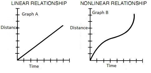
- Assumption 1: Relationship between your independent and dependent variables should always be linear i.e. you can depict a relationship between two variables with help of a straight line. Let us check whether this assumption holds true or not for our case.
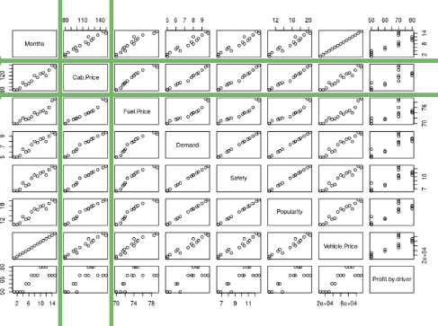
By looking at the second row and second column, we can say that our independent variables posses linear relationship(observe how scatterplots are more or less giving a shape of a line) with our dependent variable(cab price in our case)
- Assumption 2: Mean of residuals should be zero or close to 0 as much as possible. It is done to check whether our line is actually the line of “best fit”.

We want the arithmetic sum of these residuals to be as much equal to zero as possible as that will make sure that our predicted cab price is as close to actual cab price as possible. In our case, mean of the residuals is also very close to 0 hence the second assumption also holds true.
1 | |
- Assumption 4: All the dependent variables and residuals should be uncorrelated.
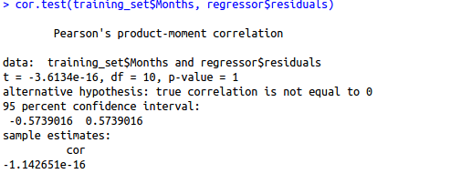
Here, our null hypothesis is that there is no relationship between our independent variable Months and the residuals while the alternate hypothesis will be that there is a relationship between months and residuals. Since the p-value is very high, we can not reject the null hypothesis and hence our assumption holds true for this variable for this model. We need to repeat this step for other independent variables also.
-
Assumption 5: Number of observations should be greater than the number of independent variables. We can check this by directly looking at our data set only.
-
Assumption 6: There should be no perfect multicollinearity in your model. Multicollinearity generally occurs when there are high correlations between two or more independent variables. In other words, one independent variable can be used to predict the other. This creates redundant information, skewing the results in a regression model. We can check multicollinearity using VIF(variance inflation factor). Higher the VIF for an independent variable, more is the chance that variable is already explained by other independent variables.
-
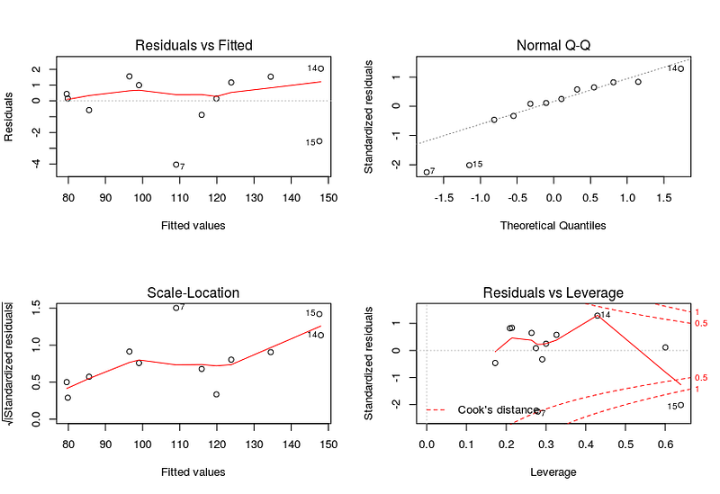
Assumption 7: Residuals should be normally distributed. This can be checked by visualizing Q-Q Normal plot. If points lie exactly on the line, it is perfectly normal distribution. However, some deviation is to be expected, particularly near the ends (note the upper right), but the deviations should be small, even lesser than they are here.
Checking assumptions automatically
We can use the gvlma library to evaluate the basic assumptions of linear regression for us automatically.
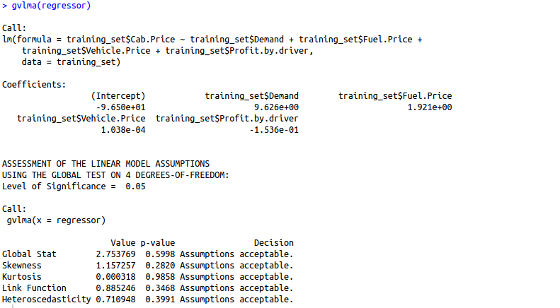

Are you finding it difficult to understand the output of the gvlma() function? Let us understand this output in detail.
1. Global Stat: It measures the linear relationship between our independent variables and the dependent variable which we are trying to predict. The null hypothesis is that there is a linear relationship between our independent and dependent variables. Since our p-value >0.05, we can easily accept our null hypothesis and conclude that there is indeed a linear relationship between our independent and dependent variables.
2. Skewness: Data can be “skewed”, meaning it tends to have a long tail on one side or the other
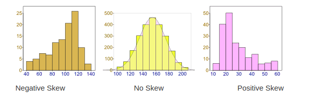
- Negative Skew: The long tail is on the “negative” (left) side of the peak. Generally, the mean < median < mode in this case.
- No Skew: There is no observed tail on any side of the peak. It is always symmetrical. Mean, median and mode are at the center of the peak i.e. mean = m0edian = mode
- Positive Skew: The long tail is on the “positive” (right) side of the peak. Generally, mode < median < mean in this case.
We want our data to be normally distributed. The second assumption looks for skewness in our data. The null hypothesis states that our data is normally distributed. In our case, since the p-value for this is >0.05, we can safely conclude that our null hypothesis holds hence our data is normally distributed.
3. Kurtosis:The kurtosis parameter is a measure of the combined weight of the tails relative to the rest of the distribution. It measures the tail-heaviness of the distribution. Although not correct, you can indirectly relate kurtosis to shape of the peak of normal distribution i.e. whether your normal distribution as a sharp peak or a shallow peak.
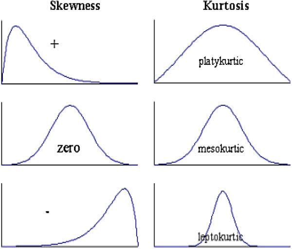
- Mesokurtic:This is generally the ideal scenario where your data has a normal distribution.
- Platykurtic(negative kurtosis score): A flatter peak is observed in this case because there are fewer data in your dataset which resides in the tail of the distribution i.e. tails are thinner as compared to the normal distribution. It has a shallower peak than normal which means that this distribution has thicker tails and that there are fewer chances of extreme outcomes compared to a normal distribution.
- Leptokurtic(positive kurtosis score):A sharper peak is observed as compared to normal distribution because there is more data in your dataset which resides in the tail of the distribution as compared to the normal distribution. It has a lesser peak than normal which means that this distribution has fatter tails and that there are more chances of extreme outcomes compared to a normal distribution.
We want our data to be normally distributed. The third assumption looks for the amount of data present in the tail of the distribution. The null hypothesis states that our data is normally distributed. In our case, since the p-value for this is >0.05, we can safely conclude that our null hypothesis holds hence our data is normally distributed.
4. Link function: It tells us whether our dependent function is numeric or categorical. As I have already mentioned before, for linear regression your dependent variable should be numeric and not categorical. The null hypothesis states that our dependent variable is numeric. Since the p-value for this case is again > 0.05, our null hypothesis holds true hence we can conclude that our dependent variable is numeric.
5. Heteroscedasticity: Is the variance of your model residuals constant across the range of X (assumption of homoskedasticity(discussed above in assumptions))? Rejection of the null (p < .05) indicates that your residuals are heteroscedastic, and thus non-constant across the range of X. Your model is better/worse at predicting for certain ranges of your X scales.
As we can observe, the gvlma function has automatically tested our model for 5 basic assumptions in linear regression and woohoo, our model has passed all the basic assumptions of linear regression and hence is a qualified model to predict results and understand the influence of independent variables (predictor variables) on your dependent variable
Understanding R squared and Adjusted R Squared
R-squared is a statistical measure of how close the data are to the fitted regression line. It is also known as the coefficient of determination, or the coefficient of multiple determination for multiple regression. It can also be defined as the percentage of the response variable variation that is explained by a linear model.
R-squared = Explained variation / Total variationR-squared is always between 0 and 100%:0% indicates that the model explains none of the variability of the response data around its mean.100% indicates that the model explains all the variability of the response data around its mean.
In general, the higher the R-squared, the better the model fits your data.But R-squared cannot determine whether the coefficient estimates and predictions are biased, which is why we must assess the residual plots. However, R-squared has additional problems that the adjusted R-squared and predicted R-squared is designed to address.

Problem 1: Whenever we add a new independent variable(predictor) to our model, R-squared value always increases. It will not depend upon whether the new predictor variable holds much significance in the prediction or not. We may get lured to increase our R squared value as much possible by adding new predictors, but we may not realize that we end up adding a lot of complexity to our model which will make it difficult to interpret.
Problem 2: If a model has too many predictors and higher order polynomials, it begins to model the random noise in the data. This condition is known as over-fitting and it produces misleadingly high R-squared values and a lessened ability to make predictions.
How adjusted R squared comes to our rescue
We will now have a look at how adjusted r squared deals with the shortcomings of r squared. To begin with, I will say that adjusted r squared modified version of R-squared that has been adjusted for the number of predictors in the model. The adjusted R-squared increases only if the new term improves the model more than would be expected by chance. It decreases when a predictor improves the model by less than expected by chance. The adjusted R-squared can be negative, but it’s usually not. It is always lower than the R-squared.
Let us understand adjusted R squared in more detail by going through its mathematical formula.
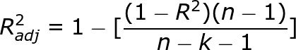
where n = number of points in our data setk = number of independent variables(predictors) used to develop the model
From the formula, we can observe that, if we keep on adding too much of non-significant predictors then k will tend to increase while R squared won’t increase so much. Hence n-k-1 will decrease and the numerator will be almost the same as before. So then entire fraction will increase(since denominator has decreased with increased k). This will result in a bigger value being subtracted from 1 and we end up with a smaller adjusted r squared value. Hence this way, adjusted R squared compensates by penalizing us for those extra variables which do not hold much significance in predicting our target variable.