
In this blog, i will try to make this concept of regression simple and intuitive for everyone. Understanding maths behind a concept is always a must before focusing on its implementation. In this part, we will try to understand what actually regression is and i will walk you through creating your first machine learning model and understanding it in and out. Hold tight because this will be something you will not wish to miss out.
Linear regression is one of the most widely known modeling technique and was the first one I learned like others while putting forward my steps in predictive learning. In this technique, the dependent variable is continuous, the independent variable(s) can be continuous or discrete, and the nature of the regression line is linear. We try to figure out a relationship between our dependent variables and independent variable using a best fitting straight line. It is called “simple” because we take only two variables in this case and try to establish a relationship between them. It is called “linear” because both the variables vary linearly (can be described with a straight line) with respect to each other. So a while plotting the relationship between two variables, we will be observing more of straight lines rather than curves.
Before diving directly into regression, let us focus on some math behind linear regression. A simple straight line can be resembled by an equation like
where y is your dependent variable**x is your independent variable or can be called regressor variable or predictor variable**m is a coefficient resembling how a unit change in x brings a change in yc is a constant which determines where your line will cut the x-axis when y=0.
To understand this relationship between our independent variable(x) and the dependent variable(y), linear regression can help us greatly.
Let us solve a problem using linear regression and understand its concepts throughout the journey
Problem: I have shifted to a new city and cab prices here from my apartment to my office are varying monthly. I want to understand the cause of these fluctuations in cab prices and if somehow I can predict what could be the price I will be paying for my cab, in the coming month
In this case, our independent variable(x) will be months and our dependent variable(y) will be the cab price. Always remember that your dependent variable is the one which you are trying to predict (cab price) and your independent variable (months) is the one which is used to predict your independent variable.
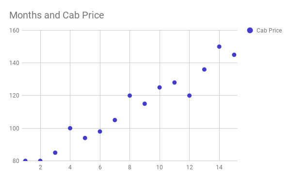
We can describe above plot roughly as
In linear regression, (in very general terms) our aim here is to find a straight line which will cover most of the points in the above graph. It is called “linear” because coefficients in this case (m) are always linear. It is good to use when your dependent and independent variables have a linear relationship i.e. it can be explained with the help of a continuous straight line
Every actual point which we have plotted is represented as Y (represented in blue)and the points which our linear regression model will predict will be termed as Y^.
Y = actual valueY^ = predicted value by model
The goal is to calculate the difference between Y and Y^ for every point, square them and sum them up for every line. Squaring the difference here solves two purposes here.1. It will heavily punish the lines which will be further away from the actual points.2. It will compensate for the actual points which lie below the regression line. (Y<Y^)The Line giving the minimum sum is chosen as the best fitting line. This method is also known as ordinary least square (OLS). This method in plain words finds from all possible fitting lines, the line with least distance from all the points.
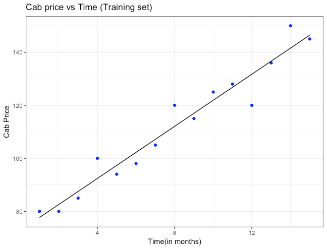
Above equation is the best fitting line which passes through most of the data points. All the blue points represent the actual cab price and the points on the line represent the predicted cab price by our linear regression model. As said previously, a best fitting line will have the least distance between the actual point and the predicted point. Now we can predict, cab price for any coming month say a 14th month from the point I have come to this new city, by just replacing month with 14 in the above equation.
Seems like i now have an estimate on how much cab price i would be paying after 2 months from now on. Hmm, interesting!
Understanding Correlation
Before building our first model, it is important to understand correlation too. Correlation is nothing but an indicator of the strength of association and relationship between two variables. In simple words, it tells you whether a certain variable will increase or decrease given a change in other variable. Value of correlation coefficient remains between -1 and 1.
-
-1 indicates a strong negative relationship between two variables
-
0 indicates no relationship between the two variables
-
+1 indicates a strong positive correlation between the two variables
Let’s take an example for each.
Strong negative correlation: Relationship between say the speed of the cab I take for office and time taken to reach office. As the speed of the cab increases, the time taken for me to reach my office decreases.
Strong positive correlation: Relationship between amount of fuel put in cab with distance it can cover. More fuel will lead it to cover further distance.
But hey, there is a small trap! I did fell into this trap when I began my career in data science and I wish to highlight that here. Keep the below line inked in your mind forever.
CORRELATION DOES NOT IMPLY CAUSATION ALWAYS
It is a very important line to keep in mind whenever you are dealing with correlation. Correlation will tell you how two variables are changing with respect to each other but one should never jump to conclusion that one is changing because of the other.
For example, last month a strong positive correlation was observed between increasing number of shark attacks and iPhone sales. It will not make any sense that increasing shark attack can lead to huge sales of iPhones.

As you can see in this graph also, with a decrease in market share of internet explorer, the murder rate has also gone down. Though it clearly states a negative correlation in no way, one can conclude that murders in the US have something to do with the fall of internet explorer market share in the US and vice-versa.

Let us not wait more and get our hands dirty with some code. We will train a simple linear regression model which will find the correlation between the two columns and by understanding that correlation, we will be finally able to predict cab prices for months to come.
Building a simple linear regression model in R
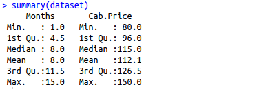
Step 1: Import the data set and use functions like summary() and colnames() to understand the data. Summary provides detailed summary of every column in your data set in R. In our data set, we have two columns i.e. Months and Cab.Price. Month is our independent variable whereas Cab.Price is the variable we are trying to predict.
1 | |
Step 2 : Split your data set into training set and test set. It is a good practice to divide your data set in such a way that you have more number of entries for your training set as compared to test set. A 75%-25% split is considered generally but it can vary accordingly in case of different scenarios.
Step 3 : Use lm function in R to build a basic simple linear regression model. First parameter (formula) requires us to write our dependent variable first then followed by “~” and then our independent variable. In second parameter(data), we pass the data object to the lm function
Step 4: It is time now to do some predictions using the model we just built. regressor object above now holds your simple linear regression model and now can be used to make predictions easily. R provides a predict function which can be used here to make predictions. It is fairly simple function which will accept your model as the first parameter and your test dataset as the second parameter
Step 5 : Visualizing your results in one of the important method to analyse your predictions. We will first try to have a look performance of our model on our training set itself to analyze its performance

Step 6 : Now let us have a look how our model has performed for our test set. First we plot all the actual points depicting cab prices with blue points on the graph. Now to compare these values with the values predicted by our model, we plot the straight line from our model which was built with the training set
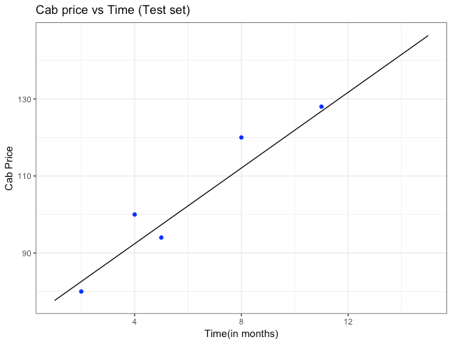
Our final model is able to predict cab price for different months and its prediction is quite closer with many values either.
Understanding our simple linear regression model
Let us deep dive into one level more to actually understand our model. Simplest way to analyze our simple linear regression model is to read result of the summary function when your model is passed as a parameter.
After executing this command, you will observe different statistics displayed in your R console. Do not get confused on seeing these different numbers and terms. Let us go through each of them one by one.
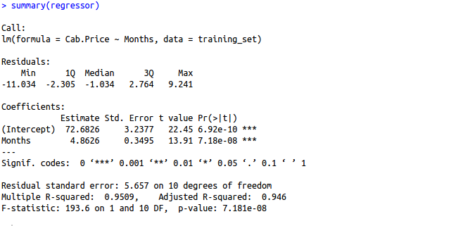
- Formula CallIt shows formula used for making the model. It displays the lm() function we used to make our simple linear regression model with Cab. Price as our dependent variable and Month as the independent variable.
- ResidualsIt is nothing but the difference in actual values which were originally present for example actual cab price in our dataset and the predicted values by the simple linear regression model. In order to analyze how well your model is fitting your data, you should look at the symmetrical distribution of these values around mean 0. In this case, values are more or less evenly distributed around 0, which implies that your model is predicting values which are closer to actual points.
- CoefficientsCoefficients are basically the values which determine how much unit change in one independent variable will lead to unit change in the dependent variable.– Estimate provides coefficients used in the actual equation of the model. Intercept estimates give value or the cab price when month value will be 0 and month intercept gives value of coefficient of the variable month. Month intercept says that for every increase in month there will be an increase of cab price by 4.914.
-
Standard Error :As we have already concluded that for every increase in month there will be an increase of cab price by 4.914(INR), i want to measure an estimate of standard difference in cab price value if we run our model again and again. By running my model multiple times, we will observe that our predicted cab price may vary by 0.331(INR)
-
T-value : The coefficient t-value is a measure of how many standard deviations our coefficient estimate is far away from 0. We want it to be far away from zero as this would indicate we could reject the null hypothesis — that is, we could declare a relationship between cab price and time exist. In our example, the t-statistic values are relatively far away from zero and are large relative to the standard error, which could indicate a relationship exists. In general, t-values are also used to compute p-values.
-
Pr>T: The Pr(>t) acronym found in the model output relates to the probability of observing any value equal or larger than t. A small p-value indicates that it is unlikely we will observe a relationship between the predictor (months) and response (cab price) variables due to chance. Typically, a p-value of5%or less is a good cut-off point. In our model example, the p-values are very close to zero. Note the ‘signif. Codes’ associated to each estimate. Three stars (or asterisks) represent a highly significant p-value. Consequently, a small p-value for the intercept and the slope indicates that we can reject the null hypothesis which allows us to conclude that there is a relationship between speed and distance.
-
Residual Standard Error :It is the average amount by which dependent variable(cab price) will deviate from true regression line. In simpler words, on average cab price in a month can vary by 5.539(INR) from the true regression line. Prediction error can also be calculated by dividing 5.539(Residual error)with 77.752(Estimate coefficient) which is around 7.12%. Also observe that this is on the basis of 13 degrees of freedom. Degree of freedom is data points that went into estimation of the dependent variable(cab price) after taking into the account the number of parameters(which are two in this case i.e. cab price and months). So degree of freedom will be 15(no. of data points)–2(no. of parameters used for prediction) = 13.
-
Multiple R-squared, Adjusted R-squared :R squared value gives the estimation of how well your model is fitting your data. It always lies between 0 and 1. 0 value will tell us that your independent variable(months) does not explain the variance present in the response variable(cab price) whereas value 1 tells us that observed variance in the response variable(cab price) can be explained by dependent variable(months). R squared value in our case is around0.9443. It means that94.43% variance found in the cab price can be explained using time(months). Generally more is the R squared, better your linear regression model. Adjusted R square is a modified type of R squared value which is used in case of multiple linear regression models as R square tends to increase with more number of independent/predictor variables. I will be discussing more about Adjusted R square and maths behind it in my next article for multiple linear regression model.
-
F-statistic :f statistic also states whether there is any relationship between predictor variable(time) and the response variable(cab price). Larger the f-statistic than 1, more the relationship between the two variables. If your data set is large then a value slightly greater than 1 is sufficient to prove the existence of relationship between predictor variable(time) and the response variable(cab price). But in the case when data set is small, value should be sufficiently higher than 1. In our case where dataset is small, f statistic value is around220 which is sufficiently large enough to prove that there exists a relationship between cab price and time(months)
So we were able to understand and build our first machine learning model and able to predict the cab price for my office ride in the coming month. We will be discussing more multiple linear regression in my next article where the cab price will not be just dependent on time but on a lot of other factors also and we will look at ways on how to accommodate these variables for our final cab price prediction. We will also look into some basic assumptions which need to be satisfied before making a linear regression model and understand over-fitting too. A lot of exciting things coming up in the next article, stay tuned!


