At Stitch Fix, we approach nearly all problems with a humans-in-the-loop framework. In some cases this means coupling algorithmic recommendations with human oversight and feedback. In others, it means building interpretable, descriptive models that provide insight to our business partners. These insights can guide and improve company decisions by providing much-needed context for the application of human expertise.
One key area of insight at Stitch Fix is the broad and complex topic of style. Mastery of this concept is required not just to put the right items into each client’s Fix, but to assist the myriad decisions the company makes: designing new products, planning our inventory assortment, assisting our stylists, generating marketing strategies, and much more. This post will walk through one approach we leverage to shed light on the world of style—matrix factorization.
Formalism
We’ll approach the concept of style starting with a simpler question: “What goes in a Fix?” This is equivalent to coming up with predicted responses for every possible item i for each user u. This response can be any feedback representing whether the user likes the aesthetic of the item. Like many companies, one key method we turn to is matrix factorization. Matrix factorization in recommendation systems can be posed simply as:
Here we are predicting the response of user u to item i with three terms—the bias of the user (how much do they like things generally?), the bias of the item (how popular is this item?), and the dot product between a k-dimensional embedding vectors of the user and the item (how well matched are this user and item?).
This framing is equivalent to a decomposition of an mxn, bias-corrected response matrix R into two far lower-dimension matrices U (mk) and (kn). Unlike many machine learning algorithms, we’re learning the implicit latent factors that compose the embeddings from raw responses instead of declaring them up front as features. Because we haven’t already observed every user-item interaction, R is sparse:
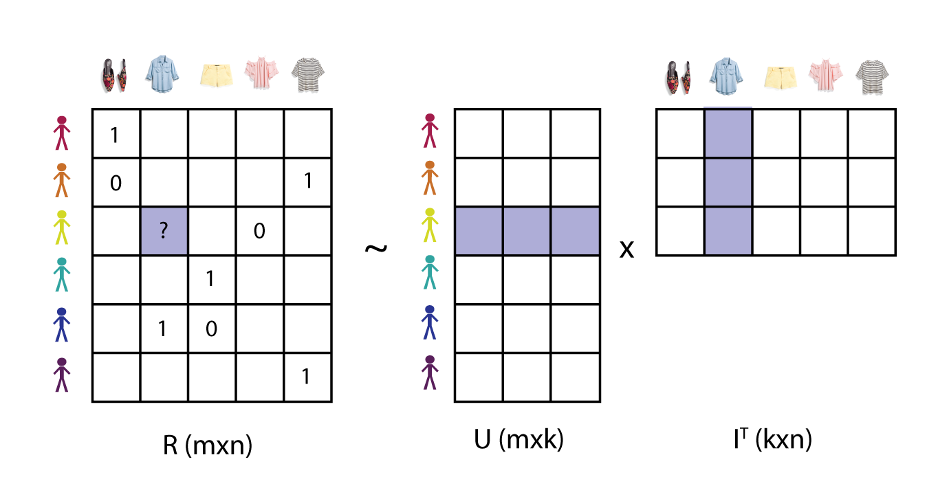
This formalism assumes there are only k latent factors that contribute to a user’s preference for an item, where k is chosen to best recover the information in our observed R. It is this assumption that reduces the complexity of this problem from on the order of (mn) to the much more tractable (k(m+n)) (though at the expense of convexity).
While (1) can be solved with a range of strategies, one common choice is to add an L2 regularization penalty to each element of and , and optimize all parameters simultaneously with stochastic gradient descent. The model can be validated with a user-conditioned AUC or rank correlation. By assessing your model with a user-conditioned metric, you ensure the model is learning more than user bias terms (an easy but often irrelevant way to improve model AUC or error).
There are many tools to choose from when solving factorization. Polylearn, lightfm, Spotlight, and Spark ALS all offer different advantages, but we turn to PyTorch for its flexibility in model specification for cases we won’t discuss here. See fuller example here.
1 | |
Interpretation
OK, so we’ve found U and I embedding matrices that are predictive of our user-item responses. We can now make recommendations to stylists of what items each client might love to have in their Fix. But how can we get a little closer to our goal of understanding style? Let’s start with some inspection of the k latent dimensions we’ve uncovered:
Before diving in, we will perform principal component analysis (PCA) on our latent embeddings. PCA will return embeddings where each component is completely independent from every other component. This orthogonality is useful for interpretability: more or less weight in one component has no impact in any other. Another plus: these new factors will be ranked by their eigenvalues, or how much variance they capture across users and items. By performing PCA on a matrix of U appended to I, we allow both users and items to define our principal axes.
Each component can be described by the placement or ordering of user and items along it. To gain intuition, let’s take a look at some of the polarizing items inhabiting the extremes of one of these axes:
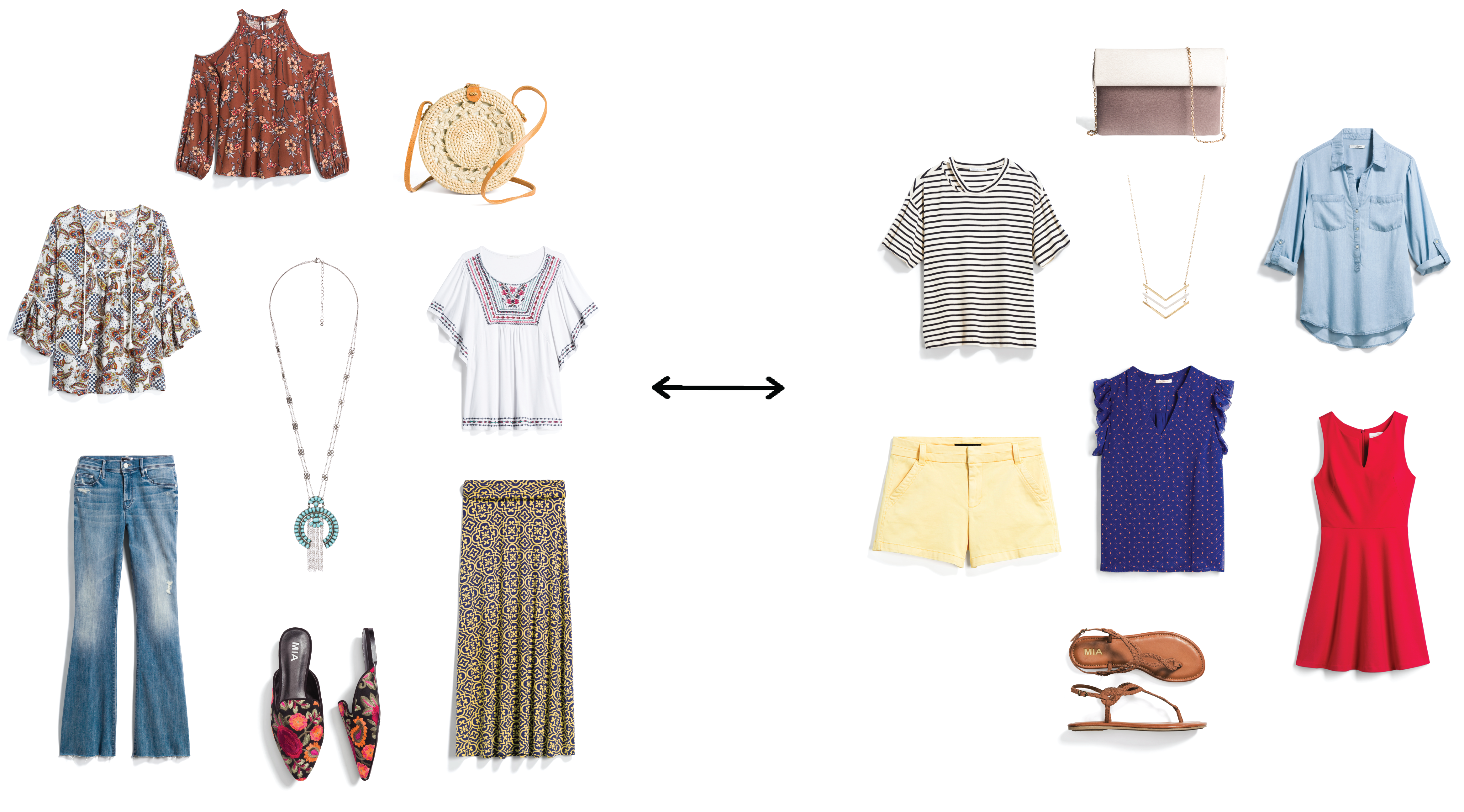
Right away, just by looking at polarizing items, we already have a sense for what’s going on here. The items with negative embedding on this axis are tile-printed, paisley, bell-sleeved, fringed, tasseled, maxi: boho. The items on the opposite end are striped, polka dotted, fitted, button-up, high chroma: preppy. A basic correlation, hypothesis test, or regression verifies this trend:
1 | |
You can do the same thing with user features and find out that users on the left side of this axis prefer Tory Burch & Lane Bryant while those on the right side prefer brands like J. Crew & Banana Republic—brands whose aesthetics map well to the characteristics above.
So now we’ve taken a step towards understanding style. Because the first component captures more variance then the second, you can think of this latent style space a bit like a decision tree. We’ve learned that the decision encountered at the first principal component is the most polarizing decision for our clients—the largest number of them lean strongly one way or another on this stylistic choice. The next principal component is our second strongest divider, and so on. A user’s predilection to like an item we offer them will be heavily influenced by this cascade of matching of the user and item along all of these axes. (Note: This tree framing holds more parallels to a hyperbolic space than a Euclidean one, but the intuition remains relevant.)
This graphic sketches out how this matching might play out under a hypothetical set of axis definitions. Try playing with the axis rankings and see how styles sort themselves. Observe how the styles sort with the default ordering of axes, then reset and try a different ordering[1].
We can now start to think about regions of this latent style space as one form of stylistic client segmentation. You can imagine solving all sorts of problems using this information: What are the design characteristics best liked by a trendy professional? We can share with our design team and vendors that black cloth, button-downs, and blazers would be good features to leverage. How many trendy boho items should we buy? We could share with our planning team what fraction of our clientele live in this region of style space, and stock accordingly. Or how about deciding whether two items are duplicative and should not both be purchased? We can calculate the item pair’s cosine similarity and surface these scores to our buyers.
Stability
There’s only one remaining hiccup left, and that’s stabilizing this latent space to a fixed reference frame. As time progresses, we will naturally have subtle shifts in the underlying assortment of our training data—different items, different clients, and evolving tastes. Additionally, factorization is a nonconvex optimization problem, so you’re not guaranteed to find a global minimum. (Though, interesting solutions to that problem exist.) The result of this is that the principal components can look a little different as time goes on. Later components that carry similar amounts of variance are particularly susceptible to being swapped and recombined. All of these small changes can result in a different basis set of vectors—the style axes would change over time. Each choice of basis set will span the space, and will likely be equally interpretable, but that interpretation process would have to be overhauled regularly.
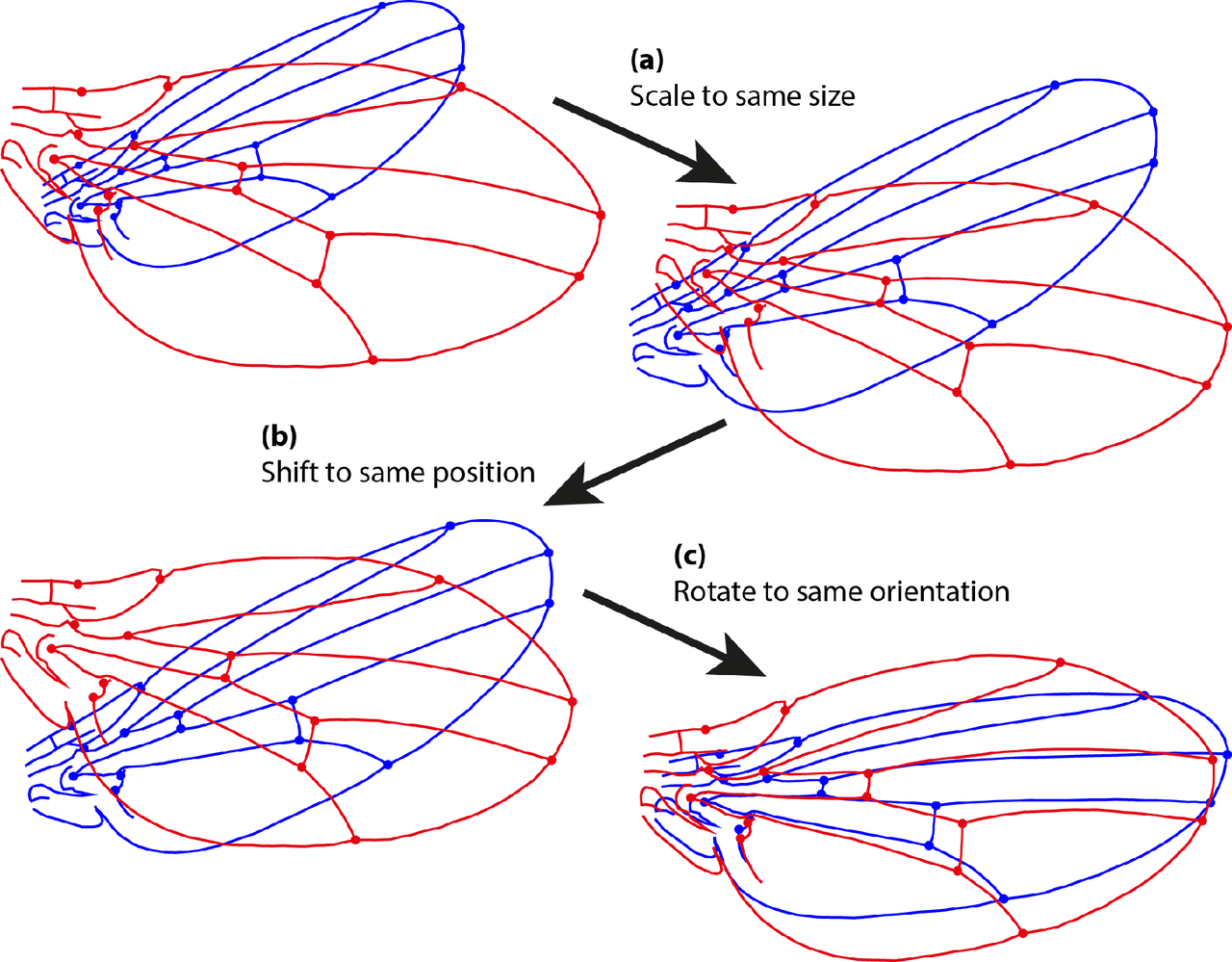
A Procrustes transformation including rescaling, care of Wikipedia Commons.
In order to avoid that process, we will rotate our latent embeddings to a fixed reference frame each time we update them—a partial Procrustes transformation: We can define as our reference embedding matrix of users and items of size . is a new embedding (potentially including new users, items, and dimensions ). To maintain interpretability, we want to find the transformation which best solves ; ie. . But, to keep predictions accurate from these embeddings we need to preserve user-item dot products. A transformation that rotates without rescaling yields both stable axes and accurate dot products, so we replace the eigenvalues of T with unity before applying it to . Simplified to only the shared users and items, this looks like: L1_inv = np.linalg.pinv(L1) T = np.dot(L1_inv, L0) u, s, v = np.linalg.svd(T) si = np.eye(u.shape[0], v.shape[0]) T_rot = np.dot(u, np.dot(si, v)) L1_rot = pd.DataFrame(np.dot(L1, T_rot), index = L1.index)
In cases where factorization is run with additional components (), the rotation will only apply to the first . By monitoring the amount of variance that ends up explained by axes, we can determine whether there are significant new latent features arising that may not have existed prior—perhaps a new trend, a seasonal component, or an expansion into a different product market. What next? There are many exciting directions to build from here. Naturally all of the correlated user and item features found above can be used to cold start users and items that haven’t yet been observed. The flexibility of PyTorch also allows for many implementations of that idea, as well as many more—temporal terms, multioutput models, highly nonlinear features, and more.
In cases where factorization is run with additional components (), the rotation will only apply to the first . By monitoring the amount of variance that ends up explained by axes, we can determine whether there are significant new latent features arising that may not have existed prior—perhaps a new trend, a seasonal component, or an expansion into a different product market.