Add Constrained Optimization To Your Toolbelt

We often make important decisions when resources are scarce.

At Stitch Fix, whenever we serve a customer, we must choose the right day to style that client’s fix, the right stylist for that client’s particular aesthetic, the right warehouse for that client’s shipping address. But stylists and warehouses are in high demand, with many clients competing for their time and attention. Constrained optimization helps us get work to stylists and warehouses in a manner that is fair and efficient, and gives our clients the best possible experience.

This post is an introduction to constrained optimization aimed at data scientists and developers fluent in Python, but without any background in operations research or applied math. We’ll demonstrate how optimization modeling can be applied to real problems at Stitch Fix. At the end of this article, you should be able to start modeling your own business problems.

Optimization Software

My constrained optimization package of choice is the python library pyomo, an open source project for defining and solving optimization problems. Pyomo is simple to install:

Pyomo is just the interface for defining and running your model. You also need a solver to do the heavy lifting. Pyomo will call out to the solver to analyze your problem, choose an appropriate algorithm, and apply that algorithm to find a solution. If you just want to get started quickly, go for GLPK, the GNu Linear Programming Kit. GLPK runs slowly on large problems but is free and dirt simple to install. On a mac:

The fastest open-source solver is CBC, but install can be a bit trickier. The commercial Gurobi software is expensive but state of the art: students and academic researchers can snag a free educational license.

Define Your Problem

Constrained optimization is a tool for minimizing or maximizing some objective, subject to constraints. For example, we may want to build new warehouses that minimize the average cost of shipping to our clients, constrained by our budget for building and operating those warehouses. Or, we might want to purchase an assortment of merchandise that maximizes expected revenue, limited by a minimum number of different items to stock in each department and our manufacturers’ minimum order sizes.

Here’s the catch: all objectives and constraints must be linear or quadratic functions of the model’s fixed inputs (parameters, in the lingo) and free variables.

Constraints are limited to equalities and non-strict inequalities. (Re-writing strict inequalities in these terms can require some algebraic gymnastics.) Conventionally, all terms including free variables live on the lefthand side of the equality or inequality, leaving only constants and fixed parameters on the righthand side.

To build your model, you must first formalize your objective function and constraints. Once you’ve expressed these terms mathematically, it’s easy to turn the math into code and let pyomo find the optimal solution.

Matching Clients and Stylists

(see it in the algorithms tour)

At Stitch Fix, our styling team styles many thousands of clients every day. Our stylists are as diverse as our clients, and matching a customer to the best suited stylist has a big impact on client satisfaction.

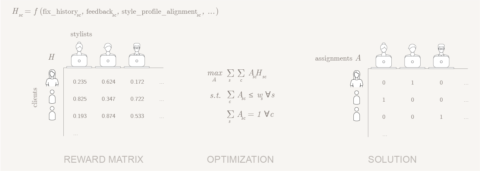
We want to match up stylists and clients in a way that maximizes the total number of happy customers, without overworking any stylist and making sure that every client gets styled exactly once. Formally, the client-stylist matching problem can be expressed as:

Where:

• is the set of all stylists working today;

• is the set of all clients we need to style today;

• is the probability that customer will be happy working with stylist ;

• is 1 if we assign stylist to work with customer and 0 otherwise; and

• is the acceptable workload of each stylist: the maximum number of clients stylist can work with today.

Here, (the matrix of happy-customer probabilities for each possible client-stylist pairing) and (the vector of acceptable workloads for each stylist) are determined by external factors. They’re known and fixed, and we don’t have any control over them. In optimization terms, they are parameters of the model.

In contrast, , the matrix of assignments, is under our complete control—within the limits defined by our constraints. We get to determine which entries are 1 and which are 0. Once we’ve coded up our model, the solver will find the values of the elements of that maximize the objective function.

Toy Scenario

Before going further, we’ll generate some toy data. Pyomo is easy to work with when data is in dictionary format, with keys treated as the named indices of a vector. For matrices, use tuples as keys, with the first element representing the row index, and the second element corresponding to the column index of the matrix.

Our toy data assigns a random chance of a happy outcome for each potential client-stylist pairing. In the real world, these values are a function of the history between the client and stylist, if any, as well as both parties’ stated and implicit style preferences.

1 2 3 4 5 6 7 8 9 10 11 12 13 14 15

import numpy as np stylist_workloads = { "Alex": 1, "Jennifer": 2, "Andrew": 2, "DeAnna": 2, "Jesse": 3} clients = ( "Trista", "Meredith", "Aaron", "Bob", "Jillian", "Ali", "Ashley", "Emily", "Desiree", "Byron") happiness_probabilities = dict( ((stylist, client), np.random.rand()) for stylist in stylist_workloads for client in clients)

Baseline

At this point, it can be useful to run a naive decision process on your data as a baseline. We tested two baseline methods on 10,000 variations of the above scenario. In the first method, assignments were made randomly. In the second method, we paired clients and stylists greedily, iteratively making the match with the highest predicted happiness probability until no clients remained or all stylists had a full workload.

Random assignment produces on average 5 happy clients, while greedy assignment averages 7.53 happy clients. If constrained optimization modeling can beat those numbers, we’ll know we’ve done useful work!

Coding Up Your Model

Once you know your objective, constraints, parameters, and variables, you can implement your model in pyomo. We begin by importing the pyomo environment and instantiating a concrete model object.

1 2 3

from pyomo import environ as pe model = pe.ConcreteModel()

Indices

In pyomo, indices are the sets of things that your parameters and variables can be defined over. In our case, that means the set of clients and the set of stylists .

We tell the model about these indices by setting fields on the model object:

1 2 3 4 5

model.stylists = pe.Set( initialize=stylist_workloads.keys()) model.clients = pe.Set( initialize=clients)

Parameters

Remember, parameters are the fixed external factors that we have no control over: the matrix of happiness probabilities for each possible client-stylist pairing, and the vector of acceptable workloads for each stylist.

In pyomo, a parameter is defined over some index. For the workload vector, that index is our set of stylists. For the happy-outcome matrix, the index is the cartesian product of the set of stylists and the set of clients: all possible client-stylist pairings.

We can also pass an argument specifying the range of values that a parameter can take. This isn’t required, but it helps the solver choose an efficient algorithm well suited to the particular optimization problem embodied by your model.

1 2 3 4 5 6 7 8 9 10 11 12 13

model.happiness_probabilities = pe.Param( # On pyomo Set objects, the '*' operator returns the cartesian product model.stylists * model.clients, # The dictionary mapping (stylist, client) pairs to chances of a happy outcome initialize=happiness_probabilities, # Happiness probabilities are real numbers between 0 and 1 within=pe.UnitInterval) model.stylist_workloads = pe.Param( model.stylists, initialize=stylist_workloads, within=pe.NonNegativeIntegers)

Variables

Next, we define our model’s free variables. Variables look similar to fixed parameters: they’re defined over some index in the model, and are restricted to some domain of possible values. The key difference is that the solver is able to manipulate the values of a variable at will. Our only variable is the assignment matrix , which can take a value of 1 when a stylist is assigned to a given client, or 0 otherwise.

1 2 3 4 5 6

model.assignments = pe.Var( # Defined over the client-stylist matrix model.stylists * model.clients, # Possible values are 0 and 1 domain=pe.Binary)

Note that the free variables in a constrained optimization problem don’t need to be binary. A different formulation of the client-stylist matching problem could assign real-valued probabilities to each possible pairing, rather than a hard 0 or 1. The merchandise-assortment example mentioned earlier would use an integer-valued variable to represent the quantity of each item we want to purchase.

Objective

We now have everything we need to express our model’s objective function: , the expected total number of happy clients that will result from our assignments. In pyomo, the summation function takes any number of parameters and variables defined over the same indices and returns an expression representing the inner product of those terms.

A pyomo Objective also specifies whether to maximize or minimize its value. In our case, we want lots of happy clients, so we’ll maximize.

1 2 3 4

model.objective = pe.Objective( expr=pe.summation(model.happiness_probabilities, model.assignments), sense=pe.maximize)

Constraints

Finally, we must tell the model about our problem’s constraints:

Like parameters and variables, pyomo constraints are defined over some index. The constraint’s rule is applied to each element in the index set. A rule is implemented as a function that takes the model and an item in the index set, and returns an equality or weak inequality constructed via a python comparison operator (==, >=, or <=). All terms of the comparison that include a model variable must live on the lefthand side of the equation.

Pyomo parameters and variables can be indexed like python dictionaries to retrieve their value for specific indices. Those values may be manipulated with standard python arithmetic operators, allowing us to easily express the constraints formulated above.

1 2 3 4 5 6 7 8 9 10 11 12 13 14 15 16 17 18 19 20 21 22 23 24 25 26 27 28 29 30 31

def respect_workload(model, stylist): # Count up all the clients assigned to the stylist n_clients_assigned_to_stylist = sum( model.assignments[stylist, client] for client in model.clients) # What's the max number of clients this stylist can work with? max_clients = model.stylist_workloads[stylist] # Make sure that sum is no more than the stylist's workload return n_clients_assigned_to_stylist <= max_clients model.respect_workload = pe.Constraint( # For each stylist in the set of all stylists... model.stylists, # Ensure that total assigned clients at most equal workload! rule=respect_workload) def one_stylist_per_client(model, client): # Count up all the stylists assigned to the client n_stylists_assigned_to_client = sum( model.assignments[stylist, client] for stylist in model.stylists) # Make sure that sum is equal to one return n_stylists_assigned_to_client == 1 model.one_stylist_per_client = pe.Constraint( # For each client in the set of all clients... model.clients, # Ensure that exactly one stylist is assigned! rule=one_stylist_per_client)

Solve It!

We’re almost done: all we need to do is apply a solver to our model and retrieve the solution.

1 2 3 4 5

# Swap out "glpk" for "cbc" or "gurobi" if using another solver solver = pe.SolverFactory("glpk") # Add the keyword arg tee=True for a detailed trace of the solver's work. solution = solver.solve(model)

Each variable in the model has a get_values() method, which, after solving, will return a mapping of indices to optimal values at that index. Variables also have a pprint() method, which will print a nicely formatted table of values—but we don’t really care about all the 0s in our assignment matrix, so let’s fish out the 1s:

1 2 3 4 5

assignments = model.assignments.get_values().items() for (stylist, client), assigned in sorted(assignments): if assigned == 1: print "{} will be styled by {}".format(client.rjust(8), stylist)

1 2 3 4 5 6 7 8 9 10 11

Desiree will be styled by Alex Ashley will be styled by Andrew Bob will be styled by Andrew Emily will be styled by DeAnna Jillian will be styled by DeAnna Aaron will be styled by Jennifer Trista will be styled by Jennifer Ali will be styled by Jesse Byron will be styled by Jesse Meredith will be styled by Jesse

Comparison to Baseline

If we run our constrained optimization model on the same 10,000 variations of the toy scenario on which we tested our random and greedy baselines, we find that our global optimization strategy produces on average 7.91 satisfied customers. That’s a 5% lift over the greedy baseline: not bad!

Final Thoughts

Constrained optimization is a tool that complements and magnifies the power of your predictive modeling skills. You’ll start to see opportunities to apply these techniques everywhere: wherever models and domain knowledge show that different resources have different costs or outcomes under different circumstances; wherever resource allocations are currently controlled by naive business rules and heuristics.

The magic lies in the problem framing. Go seek out inefficiencies. Formalize them. Optimize!