From Gaussian Algebra to Gaussian Processes, Part 2

In the previous post, we covered the following topics:

• A Gaussian process (GP) defines a distribution over functions (i.e. function evaluations). √

• Marginalizing a Gaussian over a subset of its elements gives another Gaussian (just pluck out the pieces of interest). √

• Conditioning a subset of the elements of a Gaussian on another subset gives another Gaussian (a simple algebraic formula). √

• Posterior over functions (the linear map of the posterior over weights onto some matrix (A = \phi(X_{*})^T)) √

• Covariances (the second thing we need in order to specify a multivariate Gaussian) √

If any of the above is still not clear, please look no further, and re-visit the previous post.

Conversely, we did not directly cover:

• Kernels

• Squared-exponentials

Here, we’ll explain these two.

The more features we use, the more expressive our model

We concluded the previous post by plotting posteriors over function evaluations given various phi_funcs, i.e. a function that creates “features” (\phi(X)) given an input (X).

For example:

One common such set of features are those given by “radial basis functions”, a.k.a. the “squared exponential” function, defined as:

Again, the choice of which features to use is ultimately arbitrary, i.e. a choice left to the modeler.

Throughout the exercise, we saw that the larger the dimensionality (d) of our feature function phi_func, the more expressive, i.e. less endemically prone to overfitting, our model became.

So, how far can we take this?

Computing features is expensive

Ideally, we’d compute as many features as possible for each input element, i.e. employ phi_func(x, D=some_huge_number). Unfortunately, the cost of doing so adds up, and ultimately becomes intractable past meaningfully-large values of (d).

Perhaps there’s a better way?

How are these things used?

Let’s bring back our GP equations, and prepare ourselves to squint! In the previous post, we outlined the following modeling process:

1. Define prior distribution over weights and function evaluations, (P(w, y)).

2. Marginalizing (P(w, y)) over (y), i.e. (\int P(w, y)dy), and given some observed function evaluations (y), compute the posterior distribution over weights, (P(w\vert y)).

3. Linear-mapping (P(w\vert y)) onto some new, transformed test input (\phi(X_)^T), compute the posterior distribution over function evaluations, (P(y_\ \vert\ y) = P(\phi(X_{*})^Tw\ \vert\ y)).

Now, let’s unpack #2 and #3.

(P(w\vert y))

• First, the mathematical equation:

$$\begin{align*} P(w\vert y) &= \mathcal{N}(\mu_w + \Sigma_{wy}\Sigma_y^{-1}(y - \mu_y), \Sigma_w - \Sigma_{wy}\Sigma_y^{-1}\Sigma_{wy}^T)\\ \\ &= \mathcal{N}(\mu_w + \Sigma_{wy}(\phi(X)^T\Sigma_w \phi(X))^{-1}(y - \mu_w^T \phi(X)), \Sigma_w - \Sigma_{wy}(\phi(X)^T\Sigma_w \phi(X))^{-1}\Sigma_{wy}^T) \end{align*}$$

• Next, this equation in code:

(P(y_\ \vert\ y) = P(\phi(X_{})^Tw\ \vert\ y))

Here, (X_*) is a set of test points, e.g. np.linspace(-10, 10, 200).

In addition, let’s call (X_* \rightarrow) X_test and (y_* \rightarrow) y_test.

• The mathematical equations in code:

Never alone

Squinting at the equations for mu_y_test_post and cov_y_test_post, we see that phi_x and phi_x_test appear only in the presence of another phi_x, or phi_x_test.

These four distinct such terms are:

In mathematical notation, they are (respectively):

• (\phi(X_)^T\Sigma_w \phi(X_))

• (\phi(X_*)^T\Sigma_w \phi(X))

• (\phi(X)^T\Sigma_w \phi(X))

• (\phi(X)^T\Sigma_w \phi(X_*))

Simplifying further

These are nothing more than scaled (via the (\Sigma_w) term) dot products in some expanded feature space (\phi).

Until now, we’ve explicitly chosen what this (\phi) function is.

If the scaling matrix (\Sigma_w) is positive definite, we can state the following, using (\phi(X)^T\Sigma_w \phi(X)), i.e. phi_x.T @ cov_w @ phi_x, as an example:

$$ \begin{align} \Sigma_w = (\sqrt{\Sigma_w})^2 \end{align}

$$\begin{align*} \phi(X)^T \Sigma_w \phi(X) &= \big(\sqrt{\Sigma_w}\phi(X)\big)^T\big(\sqrt{\Sigma_w}\phi(X)\big)\\ &= \varphi(X)^T\varphi(X)\\ &= \varphi(X) \cdot \varphi(X)\\ \end{align*}$$

As such, our four distinct scaled-dot-product terms can be rewritten as:

• (\phi(X_)^T\Sigma_w \phi(X_) = \varphi(X_) \cdot \varphi(X_))

• (\phi(X_)^T\Sigma_w \phi(X) = \varphi(X_) \cdot \varphi(X))

• (\phi(X)^T\Sigma_w \phi(X) = \varphi(X) \cdot \varphi(X))

• (\phi(X)^T\Sigma_w \phi(X_) = \varphi(X) \cdot \varphi(X_))

In other words, these terms can be equivalently written as dot-products in some space (\varphi).

We have not explicitly chosen what this (\varphi) function is.

Kernels

A “kernel” is a function which gives the similarity between individual elements in two sets, i.e. a Gram matrix.

For instance, imagine we have two sets of countries, ({\text{France}, \text{Germany}, \text{Iceland}}) and ({\text{Morocco}, \text{Denmark}}), and that similarity is given by an integer value in ([1, 5]), where 1 is the least similar, and 5 is the most. Applying a kernel to these sets might give a Gram matrix such as:

	France	Germany	Iceland
Morocco	4	2	1
Denmark	3	3	4

When you hear the term “kernel” in the context of machine learning, think “similarity between things in lists.” That’s it.

NB: A “list” could be a list of vectors, i.e. a matrix. A vector, or a matrix, are the canonical inputs to a kernel.

Mercer’s Theorem

Mercer’s Theorem has as a key result that any kernel function can be expressed as a dot product, i.e.

K(X, X’) = \varphi(X) \cdot \varphi (X’) $$

where (\varphi) is some function that creates (d) features out of (X) (in the same vein as phi_func from above).

Example

To illustrate, I’ll borrow an example from CrossValidated:

“For example, consider a simple polynomial kernel (K(\mathbf x, \mathbf y) = (1 + \mathbf x^T \mathbf y)^2) with (\mathbf x, \mathbf y \in \mathbb R^2). This doesn’t seem to correspond to any mapping function (\varphi), it’s just a function that returns a real number. Assuming that (\mathbf x = (x_1, x_2)) and (\mathbf y = (y_1, y_2)), let’s expand this expression:

$$\begin{align} K(\mathbf x, \mathbf y) &= (1 + \mathbf x^T \mathbf y)^2\\ &= (1 + x_1 \, y_1 + x_2 \, y_2)^2\\ &= 1 + x_1^2 y_1^2 + x_2^2 y_2^2 + 2 x_1 y_1 + 2 x_2 y_2 + 2 x_1 x_2 y_1 y_2 \end{align}$$

Note that this is nothing else but a dot product between two vectors ((1, x_1^2, x_2^2, \sqrt{2} x_1, \sqrt{2} x_2, \sqrt{2} x_1 x_2)) and ((1, y_1^2, y_2^2, \sqrt{2} y_1, \sqrt{2} y_2, \sqrt{2} y_1 y_2)), and (\varphi(\mathbf x) = \varphi(x_1, x_2) = (1, x_1^2, x_2^2, \sqrt{2} x_1, \sqrt{2} x_2, \sqrt{2} x_1 x_2)). So the kernel (K(\mathbf x, \mathbf y) = (1 + \mathbf x^T \mathbf y)^2 = \varphi(\mathbf x) \cdot \varphi(\mathbf y)) computes a dot product in 6-dimensional space without explicitly visiting this space.”

What this means

• We start with inputs (X) and (Y).

• Our goal is to compute the similarity between then, (\text{Sim}(X, Y)).

Bottom path

• Lifting these inputs into some feature space, then computing their dot-product in that space, i.e. (\varphi(X) \cdot \varphi (Y)) (where (F = \varphi), since I couldn’t figure out how to draw a (\varphi) in draw.io), is one strategy for computing this similarity.

• Unfortunately, this robustness comes at a cost: the computation is extremely expensive.

Top Path

• A valid kernel computes similarity between inputs. The function it employs might be extremely simple, e.g. ((X - Y)^{123}); the computation is extremely cheap.

Mercer!

• Mercer’s Theorem tells us that every valid kernel, i.e. the top path, is implicitly traversing the bottom path. In other words, kernels allow us to directly compute the result of an extremely expensive computation, extremely cheaply.

How does this help?

Once more, the Gaussian process equations are littered with the following terms:

• (\phi(X_)^T\Sigma_w \phi(X_) = \varphi(X_) \cdot \varphi(X_))

• (\phi(X_)^T\Sigma_w \phi(X) = \varphi(X_) \cdot \varphi(X))

• (\phi(X)^T\Sigma_w \phi(X) = \varphi(X) \cdot \varphi(X))

• (\phi(X)^T\Sigma_w \phi(X_) = \varphi(X) \cdot \varphi(X_))

In addition, we previously established that the more we increase the dimensionality (d) of our given feature function, the more flexible our model becomes.

Finally, past any meaningfully large value of (d), and irrespective of what (\varphi) actually is, this computation becomes intractably expensive.

Kernels!

You know where this is going.

Given Mercer’s theorem, we can state the following equalities:

• (\varphi(X_) \cdot \varphi(X_) = K(X_, X_))

• (\varphi(X_) \cdot \varphi(X) = K(X_, X))

• (\varphi(X) \cdot \varphi(X) = K(X, X))

• (\varphi(X) \cdot \varphi(X_) = K(X, X_))

Which kernels to choose?

At the outset, we stated that our primary goal was to increase (d). As such, let’s pick the kernel whose implicit (\varphi) has the largest dimensionality possible.

In the example above, we saw that the kernel (k(\mathbf x, \mathbf y)) was implicitly computing a (d=6)-dimensional dot-product. Which kernels compute a (d=100)-dimensional dot-product? (d=1000)?

How about (d=\infty)?

Radial basis function, a.k.a. the “squared-exponential”

This kernel is implicitly computing a (d=\infty)-dimensional dot-product. That’s it. That’s why it’s so ubiquitous in Gaussian processes.

Rewriting our equations

With all of the above in mind, let’s rewrite the equations for the parameters of our posterior distribution over function evaluations.

Defining the kernel in code

Mathematically, the RBF kernel is defined as follows:

K(X, Y) = \exp(-\frac{1}{2}\vert X - Y \vert ^2) $$

To conclude, let’s define a Python function for the parameters of our posterior over function evaluations, using this RBF kernel as k, then plot the resulting distribution.

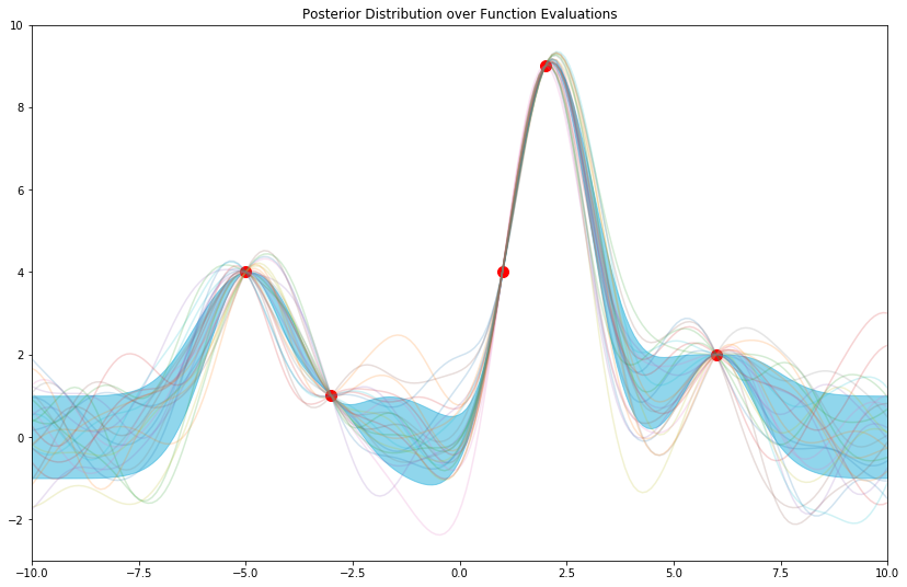
Visualizing results

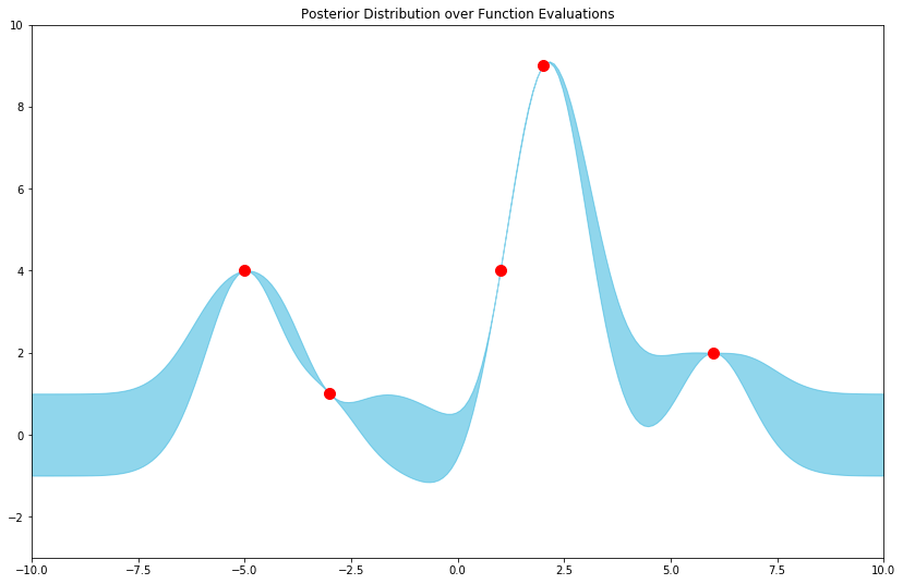
And for good measure, with some samples from the posterior:

In summary

In this post, we’ve unpacked the notion of a kernel, and its ubiquitous use in Gaussian Processes.

In addition, we’ve introduced the RBF kernel, i.e. “squared exponential” kernel, and motivated its widespread application in these models.

Code

The repository and rendered notebook for this project can be found at their respective links.

References