This article illustrates one of the practical applications of K-means clustering algorithms. Using the K-means technique, we can compress the colored image using its pixel values.
First, let’s look at how the colored images are stored. An image comprises of several very small intensity values (dots) known as Pixels. A colored image is an image that includes color information for each pixel. In a colored image, each pixel is of 3 bytes containing RGB (Red-Blue-Green) values, starting with the Red intensity value, then the Blue, then the Green intensity value for each pixel.
As you may expect, the size of a colored digital image can be huge as each pixel requires 3 bytes or (3X8) bits for recording all the intensity values. So, these images are often stored as compressed images with fewer bits for intensity values and hence, lesser memory for storage.
Formally, image compression is the type of data compression applied to digital images to reduce their cost of storage or transmission. Before moving on to the implementation, let’s go through the K-means clustering algorithm briefly.
K-means clustering is an optimization technique for finding the ‘k’ clusters or groups in a given set of data points. The data points are clustered together on the basis of some kind of similarity. Initially, it starts with the random initialization of the ‘k’ clusters and then on the basis of some similarity (like Euclidean distance metric), it aims to minimize the distance from every data point to the cluster center in each of the clusters. There are two main iterative steps to the algorithm:
a) Assignment step — Each data point is assigned to a cluster whose center is nearest to it.
b) Update step — New cluster centers (centroids) are calculated from the data points assigned to the new cluster by choosing the average value of these data points.
These iterative steps continue until the centroids stop moving further from their clusters. Now, we get several clusters separated due to some difference while some data points are grouped together due to similarity. For illustration, let’s look at the picture below. Look how the data points have been grouped according to their distance values.
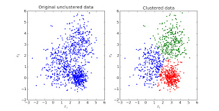 Clustered & Unclustered data
K-Means Applied On Images
In our problem of image compression, K-means clustering will group similar colors together into ‘k’ clusters (say k=64) of different colors (RGB values). Therefore, each cluster centroid is the representative of the three dimensional color vector in RGB color space of its respective cluster.
You might have guessed by now how smoothly K-means can be applied on the pixel values to get the resultant compressed image. Now, these ‘k’ cluster centroids will replace all the color vectors in their respective clusters. Thus, we need only store the label for each pixel that tells the cluster where this pixel belongs. Additionally, we keep the record of color vectors of each cluster center. Look at the original and compressed images below.
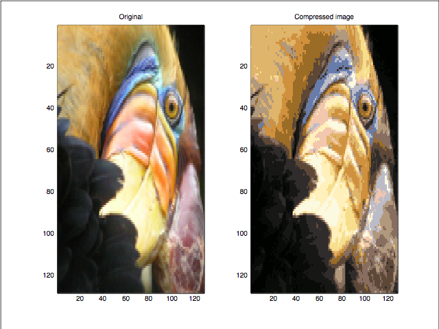
Now, lets look at whether the image is really compressed. Earlier each pixel was taking 24 (8X3) bits to store its corresponding color vector. After applying this algorithm, each pixel only takes 6 bits to do so as it only stores the label of the cluster to which it belongs (k=64 in our example). K=64 different color vectors can be represented using 6 bits only.
Thus, the resultant image will have 64 different colors in its RGB color space. Note that the compression here will be lossy (i.e. the fine details in an image may get vanished after this compression). However, we can take relatively higher values of ‘k’ to minimize this loss and make it as small as possible.
Here, we have reduced the number of colors to represent a colored digital image in a method known as Color Quantization. However, there are several different ways to achieve this target. Some other methods include reducing the size of the image, or reducing the intensity ranges of pixels, or reducing the frequency of an image.
The full MATLAB implementation of the discussed algorithm can be found on the Github link here. I recommend going through this implementation and trying it yourself as it will really solidify your concepts. If you found it helpful, please star and fork the repository.😄
Hope it was easy to follow this blog! For any further discussion on this article or any other project please leave your comments below or drop me a message on LinkedIn or Twitter. I’ll be 😄 to discuss.
Thanks for reading!