Synthetic Gradients with Tensorflow

I stumbled upon Max Jaderberg’s Synthetic Gradients paper while thinking about different forms of communication between neural modules. It’s a simple idea: rather than compute gradients through backpropagation, we can train a model to predict what those gradients will be, and use our prediction to update our weights. It’s dynamic programming for neural networks.

This is the kind of idea I like because, if it works, it expands our modeling capabilities substantially. It would allow us to connect and train various neural modules asynchronously. Whether this turns out to be useful remains to be seen. I wanted to try using this in my own work and didn’t find a Tensorflow implementation to my liking, so here is mine. I also take this opportunity to (attempt to) answer one of the questions I had while reading the paper: why not use synthetic loss instead of synthetic gradients? Supposing we had multiple paths in a DAG architecture—then a synthetic loss (or better, advantage) would give us an interpretable measure of the “quality” of a part of the input, whereas synthetic gradients do not (without additional assumptions).

Below, we use Tensorflow to implement the fully-connected MNIST experiment, as well as the convolutional CIFAR 10 experiment. The Synthetic Gradients paper itself is a non-technical and easy read, so I’m not going go into any detail about what exactly it is we’re doing. Jaderberg’s blog post may be helpful on this front. I also enjoyed Delip Rao’s blog post and follow-up.### Implementation

Imports and data

import tensorflow as tf, numpy as np, time
import matplotlib.pyplot as plt, seaborn as sns
from sklearn.utils import shuffle
%matplotlib inline
sns.set(color_codes=True)

(xtr, ytr), (xte, yte) = tf.keras.datasets.mnist.load_data(path=’mnist.npz’) xtr = xtr.reshape([-1,784]).astype(np.float32) / 255. xte = xte.reshape([-1,784]).astype(np.float32) / 255.

#### Utility functions

Note that the layer and model functions below return their variables. This is so we can do selectively compute gradients for different variables as appropriate.

def reset_graph(): if ‘sess’ in globals() and sess: sess.close() tf.reset_default_graph()

def layer_dense_bn_relu(h, size, training=True):
 l = tf.layers.Dense(size)
 h = tf.layers.batch_normalization(l(h), training=training)
 
 return tf.nn.relu(h), l.trainable_variables

def model_linear(h, output_dim, output_activation=None, 
 kernel_initializer=tf.zeros_initializer, other_inputs=None):
 """
 h is input that gets mapped to output_dim dims
 other_inputs is vector of other inputs
 """
 if other_inputs is not None:
 h = tf.concat([h, other_inputs], axis=len(h.get_shape())-1)

 l = tf.layers.Dense(output_dim, activation=output_activation, 
 kernel_initializer=kernel_initializer)
 
 return l(h), l.trainable_variables

def model_two_layer(h, output_dim, output_activation=None, 
 kernel_initializer=tf.zeros_initializer, other_inputs=None):
 """
 h is input that gets mapped to output_dim dims
 other_inputs is vector of other inputs
 """
 if other_inputs is not None:
 h = tf.concat([h, other_inputs], axis=len(h.get_shape())-1)
 
 h, v1 = layer_dense_bn_relu(h, 1024)
 h, v2 = layer_dense_bn_relu(h, 1024)
 
 l = tf.layers.Dense(output_dim, activation=output_activation, 
 kernel_initializer=kernel_initializer)
 
 return l(h), v1 + v2 + l.trainable_variables

Synthetic grad / loss wrappers and more utilities

Synthetic loss is just like synthetic gradients except we are predicting a scalar loss and then computing the gradients with respect to that loss. I thought this work similarly to the synthetic gradients, but it doesn’t seem to work at all (discussed below).

def sg_wrapper(x, h, hvs, model, other_inputs=None): 
 """
 Predicts grads for x, h, and hvs (vars between x and h) using model.
 Returns:
 - synth grad for x
 - synth grad for h
 - synth grads & vars for hvs
 - sg model variables (so they can be trained)
 """
 sg, sg_vars = model(h, h.get_shape()[-1], other_inputs=other_inputs)
 
 xs = hvs + [x]
 gvs = list(zip(tf.gradients(h, xs, grad_ys=sg), xs))
 
 return gvs[-1][0], sg, gvs[:-1], sg_vars

def sl_wrapper(h, hvs, model, other_inputs=None): 
 """
 Predicts loss given h, and produces grads_and_vars for hvs, using model.
 Returns:
 - synth loss for h
 - synth grads & vars for hvs
 - model variables (so they can be trained)
 """
 sl, sl_vars = model(h, 1, tf.square, None, other_inputs)
 gvs = list(zip(tf.gradients(sl, hvs), hvs))
 
 return sl, gvs, sl_vars

def loss_grads_with_target(loss, vs, target):
 Returns grad and vars for vs and target with respect to loss. 
 """
 xs = vs + [target]
 gvs = list(zip(tf.gradients(loss, xs), xs))
 return gvs[-1][0], gvs[:-1]

def model_grads(output_target_vars_tuple):
 """
 Returns grads and vars for models given an iterable of tuples of
 (model output, model target, model variables).
 """
 gvs = []
 for prediction, target, vs in output_target_vars_tuple:
 loss = tf.losses.mean_squared_error(prediction, target)
 gvs += list(zip(tf.gradients(loss, vs), vs))
 
 return gvs

MNIST Experiment

Note: the paper claims that the learning rate was not optimized, but I found that the results are quite sensitive to changes in the learning rate.

def build_graph_mnist_fcn(sg=False, sl=False, conditioned=False, no_bprop=False):
 reset_graph()
 g = {}
 g['training'] = training = tf.placeholder_with_default(True, [])
 
 g['x'] = x = tf.placeholder(tf.float32, [None, 784], name='x_placeholder')
 g['y'] = y = tf.placeholder(tf.int64, [None], name='y_placeholder')
 other_inputs = None
 if conditioned:
 other_inputs = tf.one_hot(y, 10)
 
 h1, h1vs = layer_dense_bn_relu(x, 256, training)
 if sg:
 _, sg1, gvs1, svars1 = sg_wrapper(x, h1, h1vs, model_two_layer, other_inputs)
 elif sl:
 sl1, gvs1, svars1 = sl_wrapper(h1, h1vs, model_two_layer, other_inputs)
 
 h2, h2vs = layer_dense_bn_relu(h1, 256, training)
 if sg:
 sg1_target, sg2, gvs2, svars2 = sg_wrapper(h1, h2, h2vs, model_two_layer, other_inputs)
 elif sl:
 sl2, gvs2, svars2 = sl_wrapper(h2, h2vs, model_two_layer, other_inputs)
 
 logit_layer = tf.layers.Dense(10)
 logits = logit_layer(h2)
 logit_vs = logit_layer.trainable_variables
 
 g['loss'] = loss =\
 tf.nn.sparse_softmax_cross_entropy_with_logits(logits=logits, labels=y)
 
 if sg:
 sg2_target, gvs3 = loss_grads_with_target(loss, logit_vs, h2)
 gvs_sg = model_grads([(sg1, sg1_target, svars1), 
 (sg2, sg2_target, svars2)])
 elif sl:
 gvs3 = list(zip(tf.gradients(loss, logit_vs), logit_vs))
 gvs_sl = model_grads([(sl1, sl2, svars1),
 (sl2, tf.expand_dims(loss, 1), svars2)])
 elif no_bprop:
 gvs3 = list(zip(tf.gradients(loss, logit_vs), logit_vs))
 
 with tf.control_dependencies(tf.get_collection(tf.GraphKeys.UPDATE_OPS)):
 opt = tf.train.AdamOptimizer(3e-5)
 if sg:
 g['ts'] =\
 opt.apply_gradients(gvs1 + gvs2 + gvs3 + gvs_sg)
 elif sl:
 g['ts'] =\
 opt.apply_gradients(gvs1 + gvs2 + gvs3 + gvs_sl)
 elif no_bprop:
 g['ts'] =\
 opt.apply_gradients(gvs3)
 else:
 g['ts'] =\
 opt.minimize(loss)
 
 g['accuracy'] = tf.reduce_mean(tf.cast(tf.equal(tf.argmax(logits, 1), y), tf.float32))
 g['init'] = tf.global_variables_initializer()
 
 return g

def train(graph, iters = 25000, batch_size = 256): g = graph res_tr = [] res_te = [] batches_per_epoch = len(xtr)//batch_size num_epochs = iters // batches_per_epoch with tf.Session() as sess: sess.run(g[‘init’]) for epoch in range(num_epochs): x, y = shuffle(xtr, ytr) acc = 0 for i in range(batches_per_epoch): feed_dict = {g[‘x’]: x[ibatch_size:(i+1)batch_size], g[‘y’]: y[ibatch_size:(i+1)batch_size]} acc_, _ = sess.run([g[‘accuracy’], g[‘ts’]], feed_dict) acc += acc_ if (i+1) % batches_per_epoch == 0: res_tr.append(acc / batches_per_epoch)

acc_te = 0 for j in range(10): feed_dict = {g[‘x’]: xte[j1000:(j+1)1000], g[‘y’]: yte[j1000:(j+1)1000], g[‘training’]: False} acc_te += sess.run(g[‘accuracy’], feed_dict) acc_te /= 10.

res_te.append(acc_te)

print(“\rEpoch {}/{}: {:4f} (TR) {:4f} (TE)”\ .format(epoch, num_epochs, acc/batches_per_epoch, acc_te), end=’’) acc = 0

return res_tr, res_te

#### Results

Below we are running only 25k iterations, which is enough to get the point (the 500k from the paper is quite excessive!).

t = time.time() g = build_graph_mnist_fcn() # baseline _, res_baseline = train(g) print(“\nTook {} seconds!”.format(time.time() - t))

Epoch 105/106: 1.000000 (TR) 0.980100 (TE)
Took 54.59836196899414 seconds!

t = time.time() g = build_graph_mnist_fcn(no_bprop=True) _, res_no_bprop = train(g) print(“\nTook {} seconds!”.format(time.time() - t))

Epoch 105/106: 0.881460 (TR) 0.889000 (TE)
Took 33.66543793678284 seconds!

t = time.time() g = build_graph_mnist_fcn(sl=True) _, res_sl = train(g) print(“\nTook {} seconds!”.format(time.time() - t))

Epoch 105/106: 0.832816 (TR) 0.842900 (TE)
Took 137.18904900550842 seconds!

t = time.time() g = build_graph_mnist_fcn(sg=True) _, res_sg = train(g) print(“\nTook {} seconds!”.format(time.time() - t))

Epoch 105/106: 0.997162 (TR) 0.977700 (TE)
Took 115.9250328540802 seconds!

t = time.time() g = build_graph_mnist_fcn(sg=True, conditioned=True) _, res_sgc = train(g) print(“\nTook {} seconds!”.format(time.time() - t))

Epoch 105/106: 0.999983 (TR) 0.980100 (TE)
Took 117.7770209312439 seconds!

plt.figure(figsize=(10,6)) plt.plot(res_baseline, label=”backprop”) plt.plot(res_no_bprop, label=”no bprop”) plt.plot(res_sg, label=”sg”) plt.plot(res_sgc, label=”sg + c”) plt.plot(res_sl, label=”sl”) plt.title(“Synthetic Gradients on MNIST”) plt.xlabel(“Epoch”) plt.ylabel(“Accuracy”) plt.ylim([0.5,1.]) plt.legend()

![](https://r2rt.com/static/images/synthetic_gradients/output_19_1.png)

The results for synthetic gradients are similar to those in the paper over the first 100 epochs (25k mini-batches).

We see that synthetic loss failed—doing worse than even the “no backpropagation” baseline (it is also the slowest approach!). This could be the result of a number of things (e.g., the loss distribution is bi-modal and hard to model, or perhaps I made a mistake in my implementation, as I did not debug extensively); I think, however, that there is something fundamentally wrong with doing gradient descent with respect to an approximated loss function. Though we might get a reasonable estimate of the loss, there is no guarantee that the gradient of our model will match the gradient of the actual loss. Imagine, for example, approximating a line with a zig-zag: one could get arbitrary good approximations but the gradient would always be wrong).

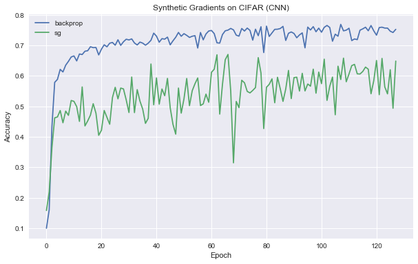
This is just to show how the implementation works with a CNN architecture. Once again, results match the paper.

(xtr, ytr), (xte, yte) = tf.keras.datasets.cifar10.load_data() xtr = xtr.astype(np.float32) / 255. ytr = ytr.reshape([-1]) xte = xte.astype(np.float32) / 255. yte = yte.reshape([-1])

def layer_conv_bn_relu(h, num_filters, filter_dim, padding="same", pooling=None, training=True):
 l = tf.layers.Conv2D(num_filters, filter_dim, padding=padding)
 h = tf.layers.batch_normalization(l(h), training=training)
 h = tf.nn.relu(h)
 
 if pooling == "max":
 h = tf.layers.max_pooling2d(h, 3, 3)
 elif pooling == "avg":
 h = tf.layers.average_pooling2d(h, 3, 3)
 
 return h, l.trainable_variables

def model_two_layer_conv(h, output_dim, other_inputs=None):
 """
 h is what we are computing the synth grads for, channels last data format
 other_inputs is vector of other inputs, assumed to have same non-channel dims
 """
 if other_inputs is not None:
 h = tf.concat([h, other_inputs], axis=len(h.get_shape())-1)
 
 h, v1 = layer_conv_bn_relu(h, 128, 5, padding="same")
 h, v2 = layer_conv_bn_relu(h, 128, 5, padding="same")
 l = tf.layers.Conv2D(output_dim, 5, padding="same", kernel_initializer=tf.zeros_initializer)
 
 return l(h), v1 + v2 + l.trainable_variables

def build_graph_cifar_cnn(sg=False): reset_graph() g = {} g[‘training’] = training = tf.placeholder_with_default(True, [])

g[‘x’] = x = tf.placeholder(tf.float32, [None, 32, 32, 3], name=’x_placeholder’) g[‘y’] = y = tf.placeholder(tf.int64, [None], name=’y_placeholder’)

h1, h1vs = layer_conv_bn_relu(x, 128, 5, ‘same’, ‘max’, training=training) if sg: _, sg1, gvs1, svars1 = sg_wrapper(x, h1, h1vs, model_two_layer_conv)

h2, h2vs = layer_conv_bn_relu(h1, 128, 5, ‘same’, ‘avg’, training=training) if sg: sg1_target, sg2, gvs2, svars2 = sg_wrapper(h1, h2, h2vs, model_two_layer_conv) h = tf.reshape(h2, [-1, 9*128])

logit_layer = tf.layers.Dense(10) logits = logit_layer(h) logit_vs = logit_layer.trainable_variables g[‘loss’] = loss = tf.nn.sparse_softmax_cross_entropy_with_logits(logits=logits, labels=y)

if sg: sg2_target, gvs3 = loss_grads_with_target(loss, logit_vs, h2) gvs_sg = model_grads([(sg1, sg1_target, svars1), (sg2, sg2_target, svars2)])

with tf.control_dependencies(tf.get_collection(tf.GraphKeys.UPDATE_OPS)): opt = tf.train.AdamOptimizer(3e-5) if sg: g[‘ts’] =\ opt.apply_gradients(gvs1 + gvs2 + gvs3 + gvs_sg) else: g[‘ts’] =\ opt.minimize(loss)

g[‘accuracy’] = tf.reduce_mean(tf.cast(tf.equal(tf.argmax(logits, 1), y), tf.float32)) g[‘init’] = tf.global_variables_initializer()

return g

t = time.time()
g = build_graph_cifar_cnn(sg=True)
res_tr, res_sg = train(g, iters=25000)
print("\nTook {} seconds".format(time.time() - t))

Epoch 127/128: 0.774700 (TR) 0.648300 (TE) Took 943.7978417873383 seconds

t = time.time()
g = build_graph_cifar_cnn() #baseline
res_tr_backprop, res_backprop = train(g, iters=25000)
print("\nTook {} seconds".format(time.time() - t))

Epoch 127/128: 0.901683 (TR) 0.752400 (TE) Took 584.2685778141022 seconds

plt.figure(figsize=(10,6))
plt.plot(res_backprop, label="backprop")
plt.plot(res_sg, label="sg")
plt.title("Synthetic Gradients on CIFAR (CNN)")
plt.xlabel("Epoch")
plt.ylabel("Accuracy")
plt.legend()