This blog post is the first in a series discussing different theoretical and practical aspects of the Frank-Wolfe algorithm.
Outline:The Frank-Wolfe AlgorithmExample: using Frank-Wolfe to solve a Lasso problemConvergence Theory
The Frank-Wolfe Algorithm
The Frank-Wolfe (FW)Originally published as Frank, Marguerite, and Philip Wolfe. “An algorithm for quadratic programming.” Naval Research Logistics (1956). See also Jaggi, Martin. “Revisiting Frank-Wolfe: Projection-Free Sparse Convex Optimization.” ICML 2013 for a more recent exposition. or conditional gradient algorithm is one of the oldest methods for nonlinear constrained optimization and has seen an impressive revival in recent years due to its low memory requirement and projection-free iterations. In its classical form, the Frank-Wolfe algorithm can solve problems of the form
\begin{equation}\label{eq:fw_objective}
\minimize_{\boldsymbol{x} \in \mathcal{M}} f(\boldsymbol{x}) ~,
\end{equation}
where $f$ is differentiable with $L$-Lipschitz gradientThis is a very standard assumption in optimization, which can be intuitively interpreted as that the objective function must be “smooth”, i.e., cannot have any kinks or discontinuities. and the domain $\mathcal{M}$ is a convex and compact set. A convex set is one for which any segment between two points lies within the set. While the FW algorithm does not require the objective function $f$ to be convex, it does require the domain to be a convex set.
Frank-Wolfe is a remarkably simple algorithm that given an initial guess $\boldsymbol{x}_0$ constructs a sequence of estimates $\boldsymbol{x}_1, \boldsymbol{x}_2, \ldots$ that converges towards a solution of the optimization problem. The algorithm is defined as follows:
\begin{align}
&\textbf{Input}: \text{initial guess $\xx_0$, tolerance $\delta > 0$}\nonumber
& \textbf{For }t=0, 1, \ldots \textbf{ do } \
&\quad\boldsymbol{s}t = \argmin{\boldsymbol{s} \in \mathcal{M}} \langle \nabla f(\boldsymbol{x}_t), \boldsymbol{s}\rangle\label{eq:lmo}\
&\quad \boldsymbol{d}_t = \ss_t - \xx_t
&\quad g_t = -\langle \nabla f(\xx_t), \dd_t \rangle
&\quad \textbf{If } g_t < \delta:
&\quad\qquad\hfill\text{// exit if gap is below tolerance }\nonumber
&\quad\qquad\textbf{return } \xx_t\
&\quad {\textbf{Variant 1}}: \text{set step size as} \nonumber\
&\quad\qquad\gamma_t = \vphantom{\sum_i}\min\Big{\frac{g_t}{L|\dd_t|^2}, 1 \Big}\label{eq:step_size}
&\quad \textbf{Variant 2}: \text{set step size by line search}\nonumber
&\quad\qquad\gamma_t = \argmin_{\gamma \in [0, 1]} f(\xx_t + \gamma \boldsymbol{d}t)\label{eq:line_search}
&\quad\boldsymbol{x}{t+1} = \boldsymbol{x}_t + \gamma_t \boldsymbol{d}_t~.\label{eq:update_rule}
&\textbf{end For loop}
& \textbf{return } \xx_t
\end{align}
Contrary to other constrained optimization algorithms like projected gradient descent, the Frank-Wolfe algorithm does not require access to a projection, hence why it is sometimes referred to as a projection-free algorithm. It instead relies on a routine that solves a linear problem over the domain (Eq. \eqref{eq:lmo}). This routine is commonly referred to as a linear minimization oracle. The rest of the algorithm mostly concerns finding the appropriate step size to move in the direction dictated by the linear minimization oracle $\dd_t = \ss_t - \xx_t$, where $\ss_t$ is the result of the linear minimization oracle. Among the many different step size rules that the FW algorithm admits, we detail two as Variant 1 and Variant 2. The first variant is easy to compute and only relies on knowledge of (a lower bound on) the Lipschitz constant $L$. The second variant instead allows to make more progress but requires to solve a 1-dimensional problem at each iteration. In some cases, such as when $f$ is a least squares loss and $\mathcal{M}$ is the $\ell_1$ norm ball, the step size selection problem has a closed form optimal solution, in which case this approach (Variant 2) should be preferred. However, in the general case this does not have a closed form solution, in which case the first variant should be preferred.
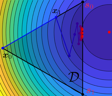
I like to see the Frank-Wolfe algorithm is as a divide-and-conquer method that transforms a potentially non-linear problem into a sequence of linear problems. It then should not come as a surprise then that its effectiveness is tightly linked to the ability to quickly solve the linear subproblems. It turns out that for a large class of problems, of which the $\ell_1$ or nuclear (also known as trace) norm ball are the most widely known examples, the linear program has either a closed form solution or efficient algorithms exist.For an extensive discussion of the cost the linear minimization oracle, see Jaggi, Martin. “Revisiting Frank-Wolfe: Projection-Free Sparse Convex Optimization.” ICML 2013. Compared to a projection, the use of a linear minimization oracle has other important consequences. For example, the output of this linear minimization oracle is always a vertex of the domainBy the properties of linear programs, the optimum value is aways attained on the boundary. and so by the update rule \eqref{eq:update_rule} the iterate is expressed as a convex combination of vertices. This feature can be very advantageous in situations with a huge or even infinite number of features, such as architecture optimization in neural networksPing W, Liu Q, Ihler AT. “Learning infinite RBMs with Frank-Wolfe”, Advances in Neural Information Processing Systems (2016). or estimation of an infinite-dimensional sparse matrix arising in multi-output polynomial networkBlondel M, Niculae V, Otsuka T, Ueda N. “Multi-output Polynomial Networks and Factorization Machines”, Advances in Neural Information Processing Systems 2017..
There are other step size strategies that I did not mention. For example, the step size can also be set as $\gamma_t = t/(t+2)$. This is an “oblivious” step size, in that it doesn’t depend on any quantity arising from the optimization. As such, it does not perform competitively in practice with the other step size strategies, although it does achieve the same theoretical rate of convergence. Another option, developed by Demyamov and RubinovDemyamov, Vladimir and Rubinov, Aleksandr “Approximate Methods in Optimization Problems”. Elsevier (1970). This is an excellent book, but unfortunately it is impossible to find online. and similar to Variant 1 is \begin{equation} \gamma_t = \min\Big{\frac{g_t}{L\,\diam(\mathcal{M})^2}, 1 \Big}~,\label{eq:step_size_diam} \end{equation} where $\diam$ denotes the diameter with respect to the euclidean norm.It is possible to use a non-euclidean norm too, as long as the Lipschitz constant $L$ is computed with respect to the same norm. For simplicity we will stick to the euclidean norm. However, since we always have $|\xx_t - \ss_t|^2 \leq \diam(\mathcal{M})^2$ by definition of diameter, the step sizes provided by this variant are always smaller than those of Variant 1 and gives a worse empirical convergence. A further improved on this step size consists in replacing the Lipschitz constant $L$ by a local estimate that can potentially be much smaller, allowing for larger step sizes. This approached is developed in our recent paper. Pedregosa, Fabian et al. “Step-size adaptivity in Projection-Free Optimization” ArXiv:1806.05123 (2018).
Yet another step size strategy that has been proposed is based on the notion of curvature constant. The curvature constant $C_f$ is defined as \begin{equation}
C_f = \sup_{\substack{\xx,\ss\in\mathcal{M},\gamma\in [0,1] \ \yy=\xx+\gamma (\ss-\xx)}} \frac{2}{\gamma^2}(f(\yy) - f(\xx) - \langle \yy - \xx, \nabla f(\xx)\rangle)
\end{equation} The curvature constant is closely related to our Lipschitz assumption on the gradient. In particular, by the definition above we always have $C_f \leq \diam(\mathcal{M})^2 L$, which given \eqref{eq:step_size_diam} suggests the following rule for the step size: \begin{equation} \gamma_t = \min\Big{\frac{g_t}{C_f}, 1 \Big}~.\label{eq:step_size_curvature} \end{equation} This step size was used for example by Lacoste-Julien 2016.Lacoste-Julien, Simon. “Convergence rate of Frank-Wolfe for non-convex objectives.” arXiv preprint arXiv:1607.00345 (2016). Note that all the results in this post are in terms of the Lipschitz constant $L$ but analogous results exist in terms of this curvature constant. The obtained rates using this curvature constant are typically tighter, however, they lead to less practical step sizes, since this constant is rarely known in practice.
Example: using Frank-Wolfe to solve a Lasso problem
Some aspects of the algorithm will become clearer with a concrete example. Lets consider a least squares problem with an $\ell_1$ constraint, a problem known as the Lasso. Given a data matrix $\boldsymbol{A} \in \RR^{n \times p}$, a target variable $\boldsymbol{b} \in \RR^n$, and a regularization parameter $\alpha$, this is a problem of the form \eqref{eq:fw_objective} with
\begin{equation}
f(\xx) = \frac{1}{2}|\boldsymbol{A}\xx - \boldsymbol{b}|^2~,\quad \mathcal{M} = {\xx : |\xx|_1\leq \alpha}
\end{equation}
In this case, the domain is a polytope and its vertices are ${\alpha e_1, -\alpha e_1, \alpha e_2, -\alpha e_2, \ldots, \alpha e_p, -\alpha e_p}$,
where $e_i$ is the $i$-th element of the canonical basis, i.e., the vector that is zero everywhere except in the $i$-th coordinate, in which it equals one.In a 2-dimensional space, the $\ell_1$ ball of radius $\alpha$ is the convex hull of its 4 vertices ${\alpha e_1, -\alpha e_1, \alpha e_2, -\alpha e_2}$, where $e_1 = (1, 0)$ and $e_2 = (0, 1)$ 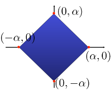 Similarly, in a $p$-dimensional space, the $\ell_1$ ball is the convex hull of ${\alpha e_1, -\alpha e_1, \alpha e_2, -\alpha e_2, \ldots, \alpha e_p, -\alpha e_p}$
The Lipschitz constant of $\nabla f$ is easy to compute, but in this precise case we can do even better, since as we will see the line search (Variant 2) option has a closed form expression. The objective function of the line search \eqref{eq:line_search} is of the form \begin{equation} f(\xx_t + \gamma \dd_t) = \frac{1}{2}|\gamma \boldsymbol{A}(\ss_t - \xx_t) + \boldsymbol{A}\xx_t - \boldsymbol{b}|^2~, \end{equation} and deriving with respect to $\gamma$ we can easily verify that the following step size solves the line search problem \begin{equation} \gamma_t = \frac{\boldsymbol{q_t}^T (\boldsymbol{b} - \boldsymbol{A} \xx)}{|\boldsymbol{q}_t|^2}~, \end{equation} with $\boldsymbol{q}_t = \boldsymbol{A}(\boldsymbol{s}_t - \xx_t)$. Below is an example in Python of the Frank-Wolfe algorithm in this case, applied to a synthetic dataset.
This simple implementation takes around 20 seconds to solve a 10.000 $\times$ 10.0000 problem (although the emphasis of this implementation is on clarity and not speed) and produces the following output:
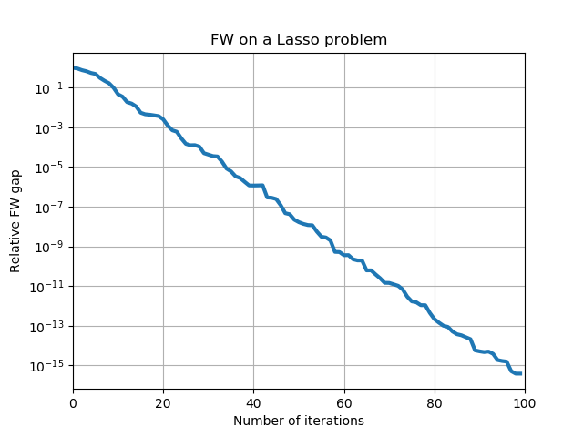
Which shows the decrease in the Frank-Wolfe gap as a function of the number of iterations. Note that although the decrease seems to be exponential, we can in general not guarantee an exponential (also known as linear) decrease rate for the Frank-Wolfe algorithm. This will only be the case for other variants such as the Away-steps Frank-Wolfe that we will discuss in upcoming posts.
1 | |
Convergence Theory
The Frank-Wolfe algorithm converges under very mild assumptions. As we will see, not even convexity of the objective is necessary to obtain weak convergence guarantees. As before, I will assume without explicit mention that $f$ is differentiable with $L$-Lipschitz gradient and $\mathcal{M}$ is a convex and compact set.
In this part I will present two main convergence results: one for general objectives and one for convex objectives. For simplicity I assume that the linear subproblems are solved exactly, but these proofs can easily be extended to consider approximate linear minimization oracles. These proofs can be found for example in Pedregosa, Fabian et al. “Step-size adaptivity in Projection-Free Optimization” ArXiv:1806.05123 (2018)..
The remainder of the section is structured as follows: I first introduce two key definition and technical Lemma, and finally prove the convergence results.
Definition 1: Stationary point. We will say that $\xx^* \in \mathcal{M}$ is a stationary point if The intuitive meaning of this definition is that $\xx^$ is a stationary point if every direction in the polytope with origin at $\xx^$ is positively correlated with the gradient. Said otherwise, $\xx^$ is a stationary point if there are no feasible descent directions with origin at $\xx^$.
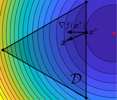
Definition 2: Frank-Wolfe gap. We denote by $g_t$ the Frank-Wolfe gap, defined as \begin{equation} g_t = \langle \nabla f(\xx_t), \xx_t - \ss_t \rangle \end{equation}
Note that by the definition of $\ss_t$ in \eqref{eq:lmo} we always have $\langle \nabla f(\xx_t), \ss_t\rangle \leq \langle \nabla f(\xx_t), \xx_t\rangle$ and so the Frank-Wolfe gap is always non-negative, and zero only at a stationary point. This makes it a good criterion to measure distance to a stationary point, and in fact convergence results for general (i.e., potentially non-convex) objectives will be given in terms of this quantity.
When $f$ is convex we also have that the FW gap verifies \begin{align}\label{eq:convexity_fw_gap}
g_t &= \max_{\ss \in \mathcal{M}}\langle \nabla f(\xx_t), \xx_t - \ss\rangle \
&\geq \langle \nabla f(\xx_t), \xx_t - \xx^\rangle
& \geq f(\xx_t) - f(\xx^)
\end{align}
where the last inequality follows from the definition of convexityA differentiable function is said to be convex if $f(\yy) \geq f(\xx) + \langle \nabla f(\xx), \yy - \xx\rangle$ for all $\xx, \yy$ in the domain.
and so can be used as a function suboptimality certificate.
The next lemma relates the objective function value at two consecutive iterates and will be key to prove convergence results, both for convex and non-convex objectives. Given its usefulness in the following I will name it “Key recursive inequality”.
Lemma 1: Key recursive inequality. Let ${\xx_0, \xx_1, \ldots}$ be the iterates produced by the Frank-Wolfe algorithm (in either variants). Then we have the following inequality, valid for any $\xi \in [0, 1]$: \begin{equation} f(\xx_{t+1}) \leq f(\xx_t) - \xi g_t + \frac{1}{2}\xi^2 L \diam(\mathcal{M})^2 \end{equation}