TSrepr - Time Series Representations in R

I’m happy to announce a new package that has recently appeared on CRAN, called “TSrepr” (version 1.0.0: https://CRAN.R-project.org/package=TSrepr).

The TSrepr package contains methods of time series representations (dimensionality reduction, feature extraction or preprocessing) and several other useful helper methods and functions.

Time series representation can be defined as follows:

Let ( x ) be a time series of length ( n ), then representation of ( x ) is a model ( \hat{x} ) with reduced dimensionality ( p ) ( (p < n) ) such that ( \hat{x} ) approximates closely ( x ) (Esling and Agon (2012)).

Time series representations are used for:

• significant reduction of the time series dimensionality

• emphasis on fundamental (essential) shape characteristics

• implicit noise handling

• reducing the dimension will reduce memory requirements and computational complexity of consequent machine learning methods.

Therefore, they are awesome!

Time series representation methods can be divided into four groups (types) (Ratanamahatana et al. (2005)):

• nondata adaptive

• data adaptive

• model-based

• data dictated (clipped data).

In nondata adaptive representations, the parameters of transformation remain the same for all time series, irrespective of their nature. In data adaptive representations, the parameters of transformation vary depending on the available data. An approach to the model-based representation relies on the assumption that the observed time series was created based on basic model. The aim is to find the parameters of such a model as a representation. Two time series are then considered as similar if they were created by the same set of parameters of a basic model. In data dictated approaches, the compression ratio is defined automatically based on raw time series such as clipped (Aghabozorgi, Seyed Shirkhorshidi, and Ying Wah (2015)).

Most famous (well known) methods for nondata adaptive type of representations are PAA (Piecewise Aggregate Approximation), DWT (Discrete Wavelet Transform), DFT (Discrete Fourier Transform), DCT (Discrete Cosine Transform) or PIP (Perceptually Important Points). For data adaptive type of representations, it is SAX (Symbolic Aggregate approXimation), PLA (Piecewise Linear Approximation) and SVD (Singular Value Decomposition). For model-based representations it is ARMA, mean profiles or estimated regression coefficients from a statistical model (e.g. linear model). The data dictated is the less known type of representation and the most famous method of this type is clipping (bit-level) representation (Bagnall et al. (2006)).

Implemented methods and functions

In the TSrepr package, these time series representation methods are implemented (the function names are in brackets):

Nondata adaptive:

• PAA - Piecewise Aggregate Approximation (repr_paa)

• DWT - Discrete Wavelet Transform (repr_dwt)

• DFT - Discrete Fourier Transform (repr_dft)

• DCT - Discrete Cosine Transform (repr_dct)

• SMA - Simple Moving Average (repr_sma)

• PIP - Perceptually Important Points (repr_pip)

• SAX - Symbolic Aggregate Approximation (repr_sax)

• PLA - Piecewise Linear Approximation (repr_pla)

• Mean seasonal profile - Average seasonal profile, Median seasonal profile, etc. (repr_seas_profile)

• Model-based seasonal representations based on linear (additive) model (LM, RLM, L1, GAM) (repr_lm, repr_gam)

• Exponential smoothing seasonal coefficients (repr_exp)

• FeaClip - Feature extraction from clipping representation (repr_feaclip, clipping)

• FeaTrend - Feature extraction from trending representation (repr_featrend, trending)

• FeaClipTrend - Feature extraction from clipping and trending representation (repr_feacliptrend)

Some additional useful functions are also implemented in the TSrepr package, such as:

• Windowing (repr_windowing) - applies to the above mentioned representations to every window of a time series

• Matrix of representations (repr_matrix) - applies to the above mentioned representations to every row of a matrix of time series

• Normalisation functions - z-score (norm_z), min-max (norm_min_max)

• Normalisation functions with output also of scaling parameters - z-score (norm_z_list), min-max (norm_min_max_list)

• Denormalisation functions - z-score (denorm_z), min-max (denorm_min_max)

• Forecasting accuracy measures - MAE, RMSE, MdAE, MAPE, sMAPE, MASE.

Usage of the TSrepr package

The TSrepr functions can be used very easily. The input is always a numeric vector (univariate time series) and additional arguments can occur in some methods.

Let’s load the package and ggplot2 for visualizations:

1 2 3

# install.packages("TSrepr") library(TSrepr) library(ggplot2)

Let’s load electricity consumption data (elec_load) and use first time series from the dataset. There is 672 values, so 14 days of measurements.

1 2 3 4 5 6

data("elec_load") data_ts <- as.numeric(elec_load[1,]) ggplot(data.frame(Time = 1:length(data_ts), Value = data_ts), aes(Time, Value)) + geom_line() + theme_bw()

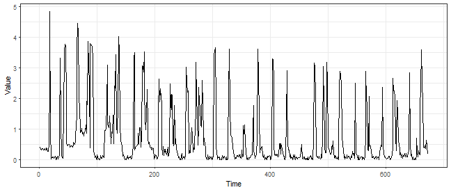
Now, we want to for example reduce dimensionality and reduce the noise of our time series. We can of course, use the time series representations from the TSrepr package. We can compare multiple methods here that are suitable for this task (smoothing of highly noised time series), for example, PAA, DWT, DFT or DCT. We will reduce dimensionality 8 times, so from 672 to 84.

1 2 3 4 5 6 7 8

# DWT with level of 2^3 data_dwt <- repr_dwt(data_ts, level = 3) # first 84 DFT coefficients are extracted and then inverted data_dft <- repr_dft(data_ts, coef = 84) # first 84 DCT coefficients are extracted and then inverted data_dct <- repr_dct(data_ts, coef = 84) # Classical PAA data_paa <- repr_paa(data_ts, q = 8, func = mean)

Let’s plot the results:

1 2 3 4 5 6 7 8

data_plot <- data.frame(Value = c(data_dwt, data_dft, data_dct, data_paa), Time = rep(1:length(data_dwt), 4), Method = factor(rep(c("DWT", "DFT", "DCT", "PAA"), each = length(data_dwt)))) ggplot(data_plot, aes(Time, Value, color = Method)) + geom_line(alpha = 0.80, size = 0.8) + theme_bw()

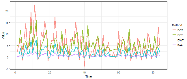
We can see that the electricity consumption pattern remains also after significant reduction of dimensionality. The difference between these four representation methods is not really significant, every one of them “did the job” well.

For seasonal time series as electricity load data, the model-based representations are highly recommended (Laurinec et al. (2016), Laurinec and Lucká (2016)). By model-based representation, we can extract a daily profile of some consumer. We can do it by simple average (or median) daily profile or by extraction of seasonal regression coefficients.

For this task, several methods are implemented in the TSrepr package. The mean seasonal profile (repr_seas_profile), seasonal linear models (repr_lm), seasonal additive model (repr_gam) or seasonal exponential smoothing coefficients (repr_exp). Let’s compare them on our data.

1 2 3 4 5 6 7 8 9

data_lm <- repr_lm(data_ts, freq = 48, method = "lm") # robust linear model and l1 regression are also implemented data_l1 <- repr_lm(data_ts, freq = 48, method = "l1") # GAM data_gam <- repr_gam(data_ts, freq = 48) # median seasonal profile data_seas_prof <- repr_seas_profile(data_ts, freq = 48, func = median) # exponential smoothing data_exp <- repr_exp(data_ts, freq = 48)

And let’s plot the results:

1 2 3 4 5 6 7 8

data_plot <- data.frame(Value = c(data_lm, data_l1, data_seas_prof, data_exp, data_gam), Time = c(rep(1:length(data_lm), 4), 1:length(data_gam)), Method = c(rep(c("LM", "L1", "Median seas. prof.", "Exp. smooth."), each = 48), rep("GAM", 47))) ggplot(data_plot, aes(Time, Value, color = Method)) + geom_line(alpha = 0.80, size = 0.8) + theme_bw()

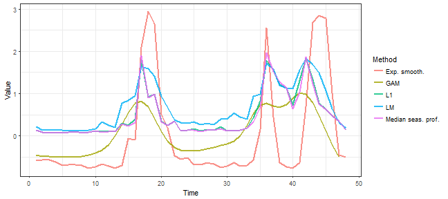
We can see that the most fluctuate result has exponential smoothing representation and the most smooth (denoised) result has seasonal GAM representation. Median daily profile and seasonal L1 regression coefficients are almost identical, the seasonal linear model regression coefficients representation is similar to them, but not that smooth.

There are also two similar time series representation methods in TSrepr package that extract important points from time series - PIP and PLA. Let’s try it on our data, and we will extract 60 points from the original time series (there will be 61 points in the end because of the nature of these methods). If we set return = "both", then data.frame with both places and points will be returned.

1 2	data_pip <- repr_pip(data_ts, times = 60, return = "both") data_pla <- repr_pla(data_ts, times = 60, return = "both")

And, of course, let’s plot the results.

1 2 3 4 5 6 7 8

data_plot <- data.frame(Value = c(data_ts, data_pip$points, data_pla$points), Time = c(1:length(data_ts), data_pip$places, data_pla$places), Method = c(rep("Original", length(data_ts)), rep(c("PIP", "PLA"), each = length(data_pla$places)))) ggplot(data_plot, aes(Time, Value, color = Method)) + geom_line(alpha = 0.65, size = 0.8) + theme_bw()

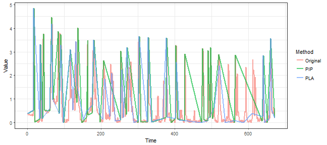
We can see some significant differences among these two methods, but both approaches identified important points well.

The next data adaptive representation method is SAX. The SAX is a famous time series representation method – for its adaptability and originality. It extracts symbols as representation, in other words, it transforms aggregates of a time series to alphabetical symbols. Let’s use it on our data:

1 2 3

# aggregates of size 12 and alphabet of size 10 repr_sax(data_ts, q = 12, a = 10)

[1] “g” “i” “g” “j” “g” “j” “j” “j” “f” “i” “j” “j” “f” “h” “j” “j” “f”

[18] “i” “h” “h” “f” “i” “i” “i” “f” “i” “f” “i” “f” “g” “g” “i” “f” “i”

[35] “g” “h” “f” “f” “f” “i” “h” “h” “f” “i” “f” “g” “f” “i” “f” “h” “g”

[52] “i” “f” “h” “g” “i”

1 2 3 4 5 6 7 8 9 10

The last type of implemented representation methods is the **data dictated** - clipped. I developed two methods in this category - **FeaClip** and **FeaTrend**. Both creates bit-level (binary) representation from original time series and computes run lengths of values by RLE (Run Length Encoding). Then interpretable features are extracted from run lengths. I will now describe the first of the mentioned methods - **FeaClip**. Clipping representation is created very easily - if a value of a time series is greater then its average value, then the value is transformed to 1 and otherwise to 0. It can be defined formally as follows: where $\mu$ is the average value of a time series. On **clipping** (bit-level) representation $\hat{x}$, compression method for binary series named Run Length Encoding (**RLE**) is applied. A run is continuous sequence of ones, respectively zeros. The number of ones respectively zeros in a run we call the run lengths. From run lengths counted by RLE, eight simple interpretable features are extracted to form the final representation and are defined as Now, I will use methods implemented in **TSrepr** package to show you how it works. The clipped series is created by function `clipping`, I will only extract the first day from the electricity consumption time series.

data_oneday <- data_ts[1:48] clipping(data_oneday)

1 2	## [1] 0 0 0 0 0 0 0 0 0 0 0 0 0 0 0 0 1 1 1 0 0 0 0 0 0 0 0 0 0 0 0 0 0 0 1 ## [36] 1 1 0 0 0 0 1 1 1 1 1 0 0

If we visualize the data with its average value, then we can see that it works as the definition above:

1 2 3 4

ggplot(data.frame(Time = 1:length(data_oneday), Value = data_oneday), aes(Time, Value)) + geom_line() + geom_line(data = data.frame(Time = 1:length(data_oneday), Value = mean(data_oneday)), aes(Time, Value), color = "red", size = 1, alpha = 0.8) + theme_bw()

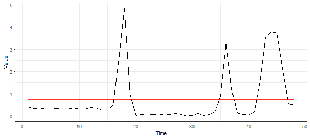
Then RLE is used for the extraction of run lengths:

rleC(clipping(data_oneday))

1 2 3 4 5

## $lengths ## [1] 16 3 15 3 4 5 2 ## ## $values ## [1] 0 1 0 1 0 1 0

And finally, the extraction of interpretable features and all previous procedures is implemented in the repr_feaclip function:

repr_feaclip(data_oneday)

1 2	## max_1 sum_1 max_0 jumps 0_1. 0_n. 1_1. 1_n. ## 5 11 16 6 16 2 0 0

The FeaClip method is recommended to use with windowing approach, so for every specified window the FeaClip computation is separately applied. For the electricity consumption data, I am using the length of the window equal to 1 day so 48 measurements. The windowing method is implemented by function repr_windowing and its arguments are representation function (func), window size (win_size) and list of additional arguments to representation function (args). Let’s use it in our case:

1 2 3 4 5

data_feaclip <- repr_windowing(data_ts, func = repr_feaclip, win_size = 48) ggplot(data.frame(Time = 1:length(data_feaclip), Value = data_feaclip), aes(Time, Value)) + geom_line() + theme_bw()

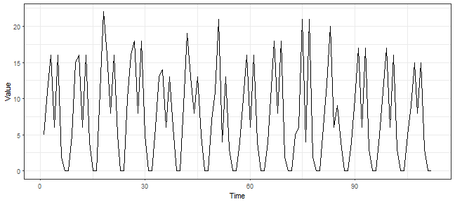
The second data dictated method is FeaTrend. It extracts features from “trending” (again binary) representation. The trending representation is defined as follows:

So, when time series value increased then it is 1, otherwise it is 0.

Before the computation of trending representation, a time series is smoothed (denoised) by simple moving average method (repr_sma) in order to have more compact run lengths. Let’s demonstrate this factor in our example case, so we will use trending and RLE function on original and also on the smoothed time series:

1 2 3

# original time series rleC(trending(data_oneday))

$lengths

[1] 2 2 2 2 1 2 2 4 2 2 1 1 1 2 2 2 1 4 4 4 4

##

$values

[1] 0 1 0 1 0 1 0 1 0 1 0 1 0 1 0 1 0 1 0 1 0

1 2 3

# smoothed time series by SMA rleC(trending(repr_sma(data_oneday, order = 4)))

$lengths

[1] 6 2 2 4 5 4 2 1 2 5 3 5 2

##

$values

[1] 0 1 0 1 0 1 0 1 0 1 0 1 0

1 2 3 4

As expected, the run lengths of smoothed time series are more compact. The **FeaTrend** is designed to extract an arbitrary feature from run lengths of a trending representation. The recommended feature is the maximum value of zeros and ones, but it can vary from an application. In the `repr_featrend` function, the windowing is directly implemented, so the original time series is divided into pieces (subseries) and features are extracted from them separately. Let’s try it in our case, but at first we will smooth original time series `data_ts` dramatically by SMA (order of moving average will be 48*7, so weekly seasonality) and do it only on whole time series (`pieces = 1`).

visualize smoothed time series

data_sma <- repr_sma(data_ts, order = 48*7) ggplot(data.frame(Time = 1:length(data_sma), Value = data_sma), aes(Time, Value)) + geom_line() + theme_bw()

1 2 3 4



compute FeaTrend representation

repr_featrend(data_ts, func = max, pieces = 1, order = 48*7)

[1] 15 30

```

So, the maximal run length of ones is 15 and maximal run length of zeros is 30, as expected, the number of zeros is much more than the number of ones because of decreasing character of the used time series.

And we have described and used every time series representation method implemented in the TSrepr package. In the next post (tutorial), I will show you one typical use case for using time series representation – clustering of time series.

References

Aghabozorgi, Saeed, Ali Seyed Shirkhorshidi, and Teh Ying Wah. 2015. “Time-series clustering - A decade review.” Information Systems 53. Elsevier: 16–38.

Bagnall, Anthony, Chotirat Ratanamahatana, Eamonn Keogh, Stefano Lonardi, and Gareth Janacek. 2006. “A bit level representation for time series data mining with shape based similarity.” Data Mining and Knowledge Discovery 13 (1): 11–40.

Esling, Philippe, and Carlos Agon. 2012. “Time-series data mining.” ACM Computing Surveys 45 (1). ACM: 1–34.

Laurinec, Peter, and Mária Lucká. 2016. “Comparison of Representations of Time Series for Clustering Smart Meter Data.” In Lecture Notes in Engineering and Computer Science: Proceedings of the World Congress on Engineering and Computer Science 2016, 458–63.

Laurinec, Peter, Marek Lóderer, Petra Vrablecová, Mária Lucká, Viera Rozinajová, and Anna Bou Ezzeddine. 2016. “Adaptive Time Series Forecasting of Energy Consumption Using Optimized Cluster Analysis.” In Data Mining Workshops (Icdmw), 2016 Ieee 16th International Conference on, 398–405. IEEE.

Ratanamahatana, Chotirat, Eamonn Keogh, Anthony J Bagnall, and Stefano Lonardi. 2005. “A Novel Bit Level Time Series Representation with Implication of Similarity Search and Clustering.” In Pacific-Asia Conference on Knowledge Discovery and Data Mining, 771–77. Springer.