I set out to write about the following paper I saw people talk about on twitter and reddit:
It’s related to this pretty insightful paper:
Inevitably, I started thinking more generally about flat and sharp minima and generalization, so rather than describing these papers in details, I ended up dumping some thoughts of my own. Feedback and pointers to literature are welcome, as always
Summary of this post
-
Flatness of minima is hypothesized to have something to do with generalization in deep nets.
-
as Dinh et al (2017) show, flatness is sensitive to reparametrization and thus cannot predict generalization ability alone.
-
Li et al (2017) use a form of parameter normalization to make their method more robust to reparametrization and produce some fancy plots comparing deep net architectures.
-
While this analysis is now invariant to the particular type of reparametrizations considered by Dinh et al, it may still be sensitive to other types of invariances, so I’m not sure how much to trust these plots and conclusions.
-
Then I go back to square one and ask how one could construct indicators of generalization that are invariant by construction, for example by considering ratios of flatness measures.
-
Finally, I have a go at developing a local measure of generalization from first principles. The resulting metric depends on the data and statistical properties of gradients calculated from different minibatches.
Flatness, Generalization and SGD
The loss surface of deep nets tends to have many local minima. Many of these might be equally good in terms of training error, but they may have widely different generalization performance, i.e. an network with minimal training loss might perform very well, or very poorly on a held-out training set. Interestingly, stochastic gradient descent (SGD) with small batchsizes appears to locate minima with better generalization properties than large-batch SGD. So the big question is: what measurable property of a local minimum can we use to predict generalization properties? And how does this relate to SGD?
There is speculation dating back to at least Hochreiter and Schmidhuber (1997) that the flatness of the minimum is a good measure to look at. However, as Dinh et al (2017) pointed out, flatness is sensitive to reparametrizations of the neural network: we can reparametrize a neural network without changing its outputs while making sharp minima look arbitrarily flat and vice versa. As a consequence the flatness alone cannot explain or predict good generalization.
Li et al (2017) proposed a normalization scheme which scales the space around a minimum in such a way that the apparent flatness in 1D and 2D plots is kind of invariant to the type of reparametrization Dinh et al used. This, they say, allows us to produce more faithful visualizations of the loss surfaces around a minimum. They even use 1D and 2D plots to illustrate differences between different architectures, such as a VGG and a ResNet. I personally do not buy the conclusions of this paper, and it seems the reviewers of the ICLR submission largely agreed on this. The proposed method is weakly motivated and only addresses one possible type of reparametrization.
Contrastive Flatness measures
Following the thinking by Dinh et al, if generalization is a property which is invariant under reparametrization, the quantity we use to predict generalization should also be invariant. My intuition is that a good way to achieve invariance is to consider the ratio between two quantities - maybe two flatness measures - which are effected by reparametrization in the same way.
One thing I think would make sense to look at is the average flatness of the loss in a single minibatch vs the flatness of the average loss. Why would this makes sense? The average loss can be flat around a minimum in different ways: it can be flat because it is the average of flat functions which all look very similar and whose minimum is very close to the same location; or it can be flat because it is the average of many sharp functions with minima at locations scattered around the minimum of the average.
Intuitively, the former solution is more stable with respect to subsampling of data, therefore it should be more favourable from a generalization viewpont. The latter solution is very sensitive to which particular minibatch we are looking at, so presumably it may give rise to worse generalization.
As a conclusion of this section, I don’t think it makes sense to look at only the flatness of the average loss, looking at how that flatness is effected by subsampling the data somehow feels more key to generalization.
A local measure of generalization
After Jorge Nocedal’s ICLR talk on large-batch SGD Leon Buttou had a comment which I think hit the nail on its head. The process of sampling minibatches from training data kind of simulates the effect of sampling the training set and the test set from some underlying data distribution. Therefore, you might think of generalization from one minibatch to another as a proxy to how well a method would generalize from a training set to a test set.
How can we use this insight to come up with some sort of measure of generalization based on minibatches, especially along the lines of sharpness or local derivatives?
First of all, let’s consider the stochastic process $f(\theta)$ which we obtain by evaluating the loss function on a random minibatch. The randomness comes from subsampling the data. This is a probability distribution over loss functions over $\theta$. I think it’s useful to seek an indicator of generalization ability as a local property of this stochastic process at any given $\theta$ value.
Let’s pretend for a minute that each draw $f(\theta)$ from this process is a convex or at least has a unique global minimum. How would one describe a model’s generalization from one minibatch to another in terms of this stochastic process?
Let’s draw two functions $f_1(\theta)$ and $f_2(\theta)$ independently (i.e. evaluate the loss on two separate minibatches). I propose that the following would be a meaningful measure:
Basically: you care about finding low error according to $f_2$ but all you have access to is $f_1$. You therefore look at what the value of $f_2$ is at the location of the minimum of $f_1$ and compare that to the global minimal value of $f_2$. This is a sort of regret expression, hence my use of $R$ to denote it.
Now, in deep learning the loss functions $f_1$ and $f_2$ are not convex, have many local minima, so this definition is not particularly useful in general. However, it makes sense to calculate this value locally, in a small neighbourhood of a particular parameter value $\theta$. Let’s consider fitting a restricted neural network model, where only parameters within a certain $\epsilon$ distance from $\theta$ are allowed. If $\epsilon$ is small enough, we can assume the loss functions have a unique global minimum within this $\epsilon$-ball. Furthermore, if $\epsilon$ is small enough, one can use a first-order Taylor-approximation to $f_1$ and $f_2$ to analytically find approximate minima within the $\epsilon$-ball. To do this, we just need to evaluate gradient at $\theta$. this is illustrated in the figure below:
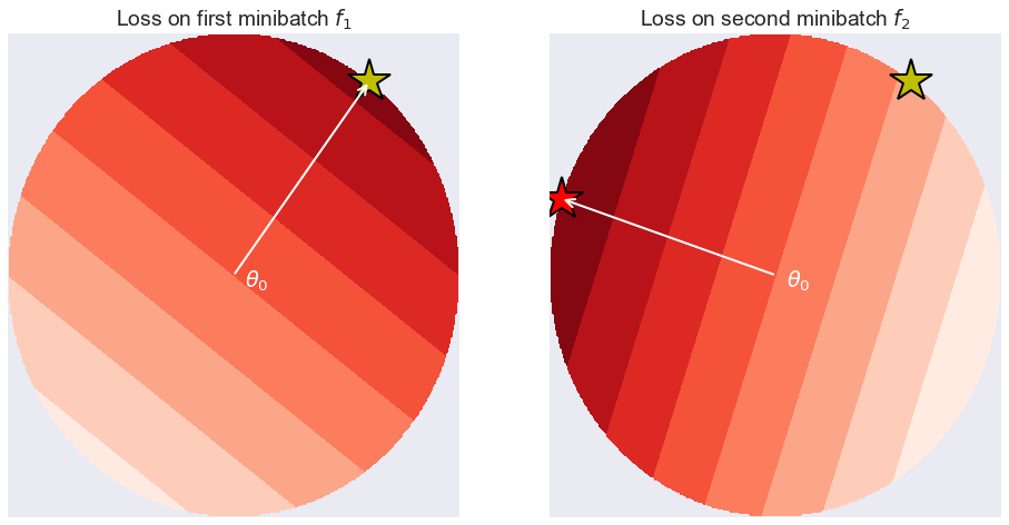
The left-hand panel shows an imaginary loss function evaluated on some minibatch $f_1$, restricted to the $\epsilon$-ball around $\theta$. We can assume $\epsilon$ is small enough so $f_1$ is linear within this local region. Unless the gradient is exactly $0$, the minimum will fall on the surface of the $\epsilon$-ball, exactly at $\theta - \epsilon \frac{g_1}{|g_1|}$ where $g_1$ is the gradient of $f_1$ at $\theta$. This is shown by the yellow star. On the right-hand panel I show $f_2$. This is also locally linear, but its gradient $g_2$ might be different. The minimum of $f_2$ within the $\epsilon$-ball is at $\theta - \epsilon \frac{g_2}{|g_2|}$, shown by the red star. We can consider the regret-type expression as above, by evaluating $f_2$ at the yellow star, and substracting its value at the red star. This can be expressed as follows (I divided by $\epsilon$):
\frac{R(\theta, f_1, f_2)}{\epsilon} \rightarrow - \frac{g_2^\top g_1}{|g_1|} + \frac{g_2^\top g_2}{|g_2|} = |g_2| - \frac{g_2^\top g_1}{|g_1|} = |g_2|(1 - cos(g_1, g_2)) $$
In practice one would consider taking an expectation with respect to the two minibatches to obtain an expression that depends on $\theta$. So, we have just come up with a local measure of generalization ability, which is expressed in terms of expectations involving gradients over different minibatches. The measure is local as it is specific for each value of $\theta$. It is data-dependent in that it depends on the distribution $p_\mathcal{D}$ from which we sample minibatches.
This measure depends on two things:
-
the expected similarity of gradients which come from different minibatches $1 - cos(g_1, g_2)$ looks at whether various minibatches of data push $\theta$ in similar directions. In regions where the gradients are sampled from a mostly spherically symmetric distribution, this term would be close to $1$ most of the time.
-
the magnitude of gradients $|g_2|$. Interestingly, one can express this as $\sqrt{\operatorname{trace}\left(g_2 g_2^\top\right)}$.
When we take the expectation over this, assuming that the cosine similarity term is mostly $1$ we end up with the expression $\mathbb{E}_g \sqrt{\operatorname{trace}\left(g g_2^\top\right)}$ where the expectation is taken over minibatches. Note that the trace-norm of the empirical Fisher information matrix $\sqrt{ \operatorname{trace} \mathbb{E}_g \left(g g_2^\top\right)}$ can be used as a measure of flatness of the average loss around minima, so there may be some interesting connections there. However, due to Jensen’s inequality the two things are not actually the same.
Update - thanks for reddit user bbsome for pointing this out:
Note that R is not invariant under reparametrization either. The source of this sensitivity is the fact that I considered an $\epsilon$-ball in Euclidean norm around $\theta$. The right way to get rid of this is to consider an $\epsilon$-ball using the symmetrized KL divergence as instead of the Euclidean norm, similarly to how natural gradient methods can be derived. If we do this, the formula becomes dependent only on the functions the neural network implements, not on the particular choice of parametrization. I leave it as homework for people to work out how this would change the formulae.
This post started out as a paper review, but in the end I didn’t find the paper too interesting and instead resorted to sharing ideas about tackling the generalization puzzle a bit differently. It’s entirely possible that people have done this analysis before, or that it’s completely useless. In any case, I welcome feedback.
The first observation here was that a good indicator may involve not just the flatness of the average loss around the minimum, but a ratio between two flatness indicators. Such metrics may end up invariant under reparametrization by construction.
Taking this idea further I attempted to develop a local indicator of generalization performance which goes beyond flatness. It also includes terms that measure the sensitivity of gradients to data subsampling.
Because data subsampling is something that occurs both in generalization (training vs test set) and in minibatch-SGD, it may be possible that these kind of measures might shed some light on how SGD enables better generalization.