· Read in 8 minutes · 1481 words · All posts in series ·
A probability on its own is often an uninteresting thing. But when we can compare probabilities, that is when their full splendour is revealed. By comparing probabilities we are able form judgements; by comparing probabilities we can exploit the elements of our world that are probable; by comparing probabilities we can see the value of objects that are rare. In their own ways, all machine learning tricks help us make better probabilistic comparisons. Comparison is the theme of this post—not discussed in this series before—and the right start to this second sprint of machine learning tricks.
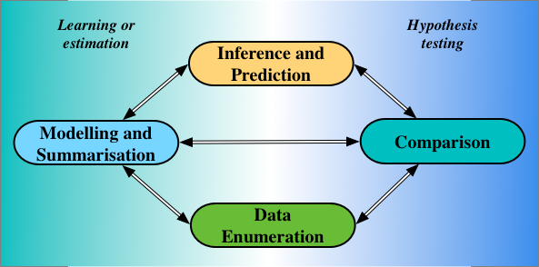
Relationship between four statistical operations [1].
In his 1981 Wald Memorial Lecture [1], Bradley Efron described four statistical operations, which remain important today: enumeration, modelling, comparison, and inference.
-
Data Enumeration is the process of collecting data (and involves systems, domain experts, and critiquing the problem at hand).
-
Modelling, or summarisation *as Efron said, *combines the ‘small bits of data’ (our training data) to extract its underlying trends and statistical structure.
-
Comparison does the opposite of modelling: it pulls apart our data to show the differences that exist in it.
-
Inferences are statements about parts of our models that are unobserved or latent, while predictions are statements of data we have not observed.
The statistical operations in the left half of the image above are achieved using the principles and practice of learning, or estimation. Those on the right half by hypothesis testing. While the preceding tricks in this series looked at learning problems, thinking instead of testing, and of statistical comparisons, can lead us to interesting new tricks.
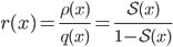
To compare two numbers, we can look at either their difference or their ratio. The same is true if we want to compare probability densities: either through a density difference or a* density ratio*. Density ratios are ubiquitous in machine learning, and will be our focus. The expression:

is the density ratio of two probability densities  and
and  of a random variable
  . This ratio is intuitive and tells us the amount by which we need to correct *q *for it to be equal to
  , since
 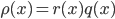 .
.
The density ratio gives the correction factor needed to make two distributions equal.
From our very first introductions to statistics and machine learning, we met such ratios: in the rules of probability, in estimation theory, in information theory, when computing integrals, learning generative models, and beyond [2][3][4].
Bayes’ Theorem
The computation of conditional probabilities is one of first ratios we encountered:
Divergences and Maximum Likelihood
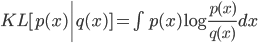
The KL divergence is the divergence most widely used to compare two distributions, and is defined in terms of a log density-ratio. Maximum likelihood is obtained by the minimisation of this divergence, highlighting how central density ratios are in our statistical practice.
Importance Sampling
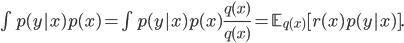
Importance sampling gives us a way of changing the distribution with respect to which an expectation is taken, by introducing an identity term and then extracting a density ratio. The ratio that emerges is referred to as an importance weight. Using 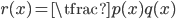 , we see that:
Mutual Information
The mutual information, a multivariate measure of correlation, is a core concept of information theory. The mutual information between two random variables x, y makes a comparison of their joint dependence versus independence. This comparison is naturally expressed using a ratio:

Hypothesis Testing
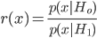
The classic use of such ratios is for hypothesis testing. The Neyman-Pearson lemma motivates this best, showing that the most powerful tests are those computed using a likelihood ratio. To compare hypothesis  (the null) to
  (the alternative), we compute the ratio of the probability of our data under the different hypotheses. The hypothesis could be two different parameter settings, or even different models.
The central task in the above five statistical quantities is to efficiently compute the ratio  . In simple problems, we can compute the numerator and the denominator separately, and then compute their ratio. Direct estimation like this will not often be possible: each part of the ratio may itself involve intractable integrals; we will often deal with high-dimensional quantities; and we may only have samples drawn from the two distributions, not their analytical forms.
This is where the density ratio trick or formally, density ratio estimation, enters: it tells us to construct a binary classifier  that distinguishes between samples from the two distributions*. *We can then compute the density ratio using the probability given by this classifier:
To show this, imagine creating a data set of 2N elements consisting of pairs (data x, label y):
By this construction, we can write the probabilities  in a conditional form; we should also keep Bayes’ theorem in mind.

We can do the following manipulations:
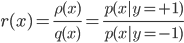
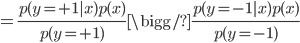
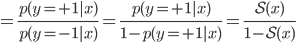
In the first line, we rewrote with ratio problem as a ratio of conditionals using the dummy labels y, *which we introduced to identify samples from the each of the distributions. In the second line, we *used Bayes’ rule to express the conditional probabilities in their inverse forms. In the final line, the marginal distributions  are equal in the numerator and the denominator and cancel. Similarly, because we used an equal number of samples from the two distributions, the prior probability
  and also cancels; we can easily include this prior to allow for imbalanced datasets. These cancellations lead us to the final line.
This final derivation says that the problem of density ratio estimation is equivalent to that of binary classification. All we need do is construct a classifier that gives the probability of a data point belonging to distribution
, and knowing that probability is enough to know the density ratio. Fortunately, building probabilistic classifiers is one of the things we know how to do best.
The idea of using classifiers to compute density ratios is widespread, and my suggestions for deeper understanding include: