When Bayesian optimization meets the Stochastic Gradient Descent algorithm on the AWS marketplace, rich features bloom, models are trained, Time-To-Market shrinks and stakeholders are satisfied.
In this article, we present an AWS based framework which allows non technical people to build predictive pipelines in a matter of hours while achieving results that rival solutions handcrafted by data scientists. This data flow revolves around two online services: Amazon’s own Machine Learning service for model training and selection and Predicsis.ai, a service available on the AWS marketplace, for feature engineering.
As the saying goes, to hire data scientists call it machine learning, to raise money call it Artificial intelligence and data science in all other cases. Whatever name you give to predictive analytics, it is the new gold rush for companies across all industries. This revolution impacts the way we communicate, trade and interact with the world. It’s a new golden age of cybernetics that we have just begun to explore. But predictive analytics takes time and can be frustrating. Expectations are high and with a bullish job market, expertise is scarce. Predictive analytics workflows require a mix of domain knowledge, data science expertise, and software proficiency that not only can be difficult to assemble but which are also challenging to bring to production. Data scientist may be the sexiest job of the early 21st century, but it will be a few years before the surging new education programs from bootcamps to college degrees, bring enough data scientists to the market. Companies don’t have the luxury to wait as competition gears up.
Within that context, AutoML offers a way to shorten project delivery time and reduce the need for junior data scientists. Before presenting these 2 services, let’s see where they fit in within the different phases of a data science project.
A typical data science workflow can be framed as following these 7 steps:
-
Business: start with a business question, define the goal and measure of success
-
Data: find, access and explore the data
-
Features: extract, assess and evaluate, select and sort
-
Models: find the right model for the problem at hand, compare, optimize, and fine tune
-
Communication: Interpret and communicate the results
-
Production: transform the code into production ready code, integrate into current ecosystem and deploy
-
Maintain: adapt the models and features to the evolution of the environment
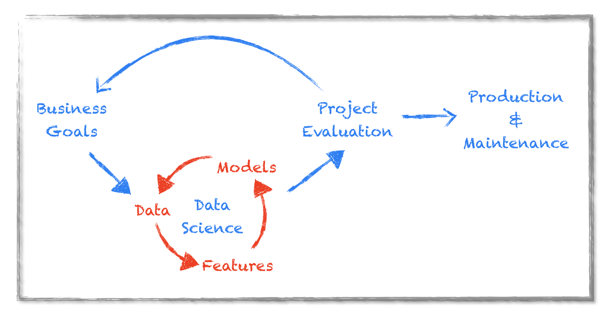
This workflow is not linear. Many iterations are necessary before first results can be interpreted and evaluated by the business. Business assessment of the results trigger new expectations and sends the team back to work on data, features and models. Finally after several such iterations, the research code is ready to be refactored for production.
Feature engineering and model selection are the most resource intensive phases and the hardest to plan for. These two phases require data science expertise in order to tackle inherent data problems such as outliers, missing values, skewed distributions and make sure the models don’t overfit through cross validation and hyper-parameter tuning.
Two services available in the AWS ecosystem can help businesses reduce their needs for data science skills and speed up the discovery phase of the data science workflow: Predicsis.ai and AWS Machine Learning.
Launched in April 2015, Amazon’s Machine Learning service, aims at “putting data science in reach of any developer”. AWS ML greatly simplifies the model training, optimization and selection phases by limiting the choice of available models to a unique one, the stochastic gradient descent (SGD). By offering parameter tuning via a simple web interface, AWS ML further simplifies the modeling step while maintaining a very high predictive performance. A simple UI, and a simple yet powerful model is the key to a very efficient modeling process. The SGD is a veteran algorithm whose conception started in the 1950’s with a seminal paper by Robbins and Monro titled A Stochastic approximation Method. The SGD has been studied and optimized extensively since then. It is powerful and robust.
AWS ML goes beyond the modeling phase of the project by offering production ready endpoints with a simple click. Thus removing the need for resource intensive code development.
However, before we can train a predictive model, we need to extract the variables from the raw data having the biggest predictive potential. This feature extraction phase is the most unpredictable and often requires expert domain knowledge. Schemes quickly become over complicated and it’s easy to end up with thousands of variables in the hope of increasing prediction performances. While trying to keep the total number of variables down, an unavoidable constraint in order to prevent overfitting.
This is where Predicsis.ai steps in by boiling down the complexity of the feature engineering phase to a few clicks through smart bayesian optimization of the feature space. Being able to automatically discover the variables that are the most predictive of the outcome, again via a simple web interface, is a game changer in a predictive analytics project. Predicsis.ai is available on the AWS marketplace. It is the de facto companion to the AWS Machine Learning service and has been selected as a key machine learning provider at the recent AWS:reInvent 2017.
With these two services in mind, the entire predictive analytics pipeline now boils down to:
-
Build the raw dataset
-
Transform it into a powerful training dataset with Predicsis.ai
-
Use that dataset to train a model on AWS ML
-
Create an endpoint for production with AWS ML
With AWS ML and Predicsis.ai, building a predictive pipeline from raw data to production endpoints can now be done in a few hours by team members wit no data science skills. People from the sales or marketing department can explore, assess and create efficient pipelines for their prediction targets.
The AWS ML service is well documented. We will focus here on Predicsis.ai and its use of bayesian optimization to build feature rich datasets. AutoML is what drives Predicis.ai.
AutoML means several things for different people but overall, AutoML is considered to be about algorithm selection, hyperparameter tuning of the model, iterative modeling, and model assessment. Without claims of exhaustivity, some of the currently available AutoML platforms and actors are:
-
H2O’s AutoML which automates the process of training a large selection of candidate prediction models.
-
Auto-sklearn which recently won the ChaLearn Automatic Machine Learning Challenge. Auto-sklearn is built on top of scikit-learn and includes 15 ML algorithms, 14 preprocessing methods, and all their respective hyperparameters, for a total of 110 hyperparameters and optimizes hyperparameter selection through bayesian optimization.
-
TPOT automatically optimizes a series of feature preprocessors and models that maximize the cross-validation accuracy on the data set. It is also scikit-learn compatible.
-
A precursor of AutoML is Auto-WEKA which considers the problem of simultaneously selecting a learning algorithm and setting its hyperparameters
-
And of course DataRobot, a leader in automated machine learning
To recapitulate, these AutoML libraries focus on optimizing
-
the model selection: deciding whether to choose an SVM over a random forest of a gradient boosted machine.
-
the hyperparameters tuning: which kernel should be used for the SVM, how to set the learning rate for the Stochastic Gradient Descent or the number of trees for the random forest?
and in some cases
- the transformations to be applied on the training data: should the data be one hot encoded or normalized through a box-cox transformation?
While these approaches are very powerful to create powerful models, we are still left with the task of engineering the most predictive variables straight out of the raw data. The challenge is even more complex when dealing with hierarchical data.
Consider for instance the case of predicting a potential buyer behavior based on three different sources: the customer’s current demographic profile, a trace of that person’s online behavior and a history of communication through emails and texts. We could probably also add that person’s social network activities, or emails or geolocation to the dataset. These different datasets come from different sources that can be aggregated to form a global customer centric hierarchical dataset. For a single person we end up with a complex mix of many variables that come in all forms and shapes: categories, flags, tags, continuous values as well as text and time series. The potential feature space expands very quickly.
Having such a large feature space triggers several problems such as multi-collinearity, overfitting and what is known as the curse of dimensionality where the feature space becomes too sparse for the algorithm to be able to effectively infer the right signal for predictions. On top of that, there’s always the potential for a yet undiscovered mix of variables to hold even better predictive potential than the ones already engineered.
If we want to reduce the time it takes to engineer and score these different variables mix, we need to automate the construction of variables. The good news is that we can adapt the model centric AutoML approach to the feature space. In other words, the bayesian approach to hyper parameter tuning can also be applied to the feature space with the goal of having a concise and powerful training dataset.
Bayesian based feature optimization is presented in the paperTowards Automatic Feature Construction for Supervised Classification by Marc Boullé from Orange Labs. The process can be decomposed as follows:
-
Define an initial feature space from the original raw hierarchical data.
-
Extend the initial feature space by applying a pre-defined series of transformations on the data.
-
Score the variables using an evaluation criterion of the constructed variables using a Bayesian approach
-
Filter out variables that score below 0 (worse than random).
With that approach it becomes possible to use all the available data as input, set the dimension of the overall feature space considered for evaluation and dictate the final number of features in the expected training dataset. This is exactly what Predicsis.ai allows. That optimized training dataset is then fed to the AWS ML service for model training and selection.
We will now show how to use Predicsis.ai in combination with AWS ML to implement a buyer prediction model based on multi-relational data. The raw data is extracted from 4 tables:
-
The Master table holds the customer’s profile information with demographic data as well as purchase history
-
The Orders table has order information (status, amount, web site, …) as well as the user’s web signature (OS, browser, mobile, …)
-
The Emails table holds email campaign related information (campaign name, recipient action, …)
-
The Visited Pages table where the customer’s online behavior is recorded.
From that data, we want to predict whether the customer will buy again from our store. The outcome corresponds to the LABEL column in the Master file. The whole dataset can be downloaded here. We will first build the optimized dataset via Predicsis.ai and then use that dataset to train a model on AWS ML.
As mentioned before, Predicsis.ai is available on the AWS Marketplace but you can also try out Predicsis.ai feature optimization by signing up for a free trial on their website. To try out AWS marketplace version of Predicsis.ai:
-
Login to your AWS account and go to the AWS marketplace Predicsi.ai page
-
Start the EC2 instance.
-
Copy the instance’s url into your favorite browser
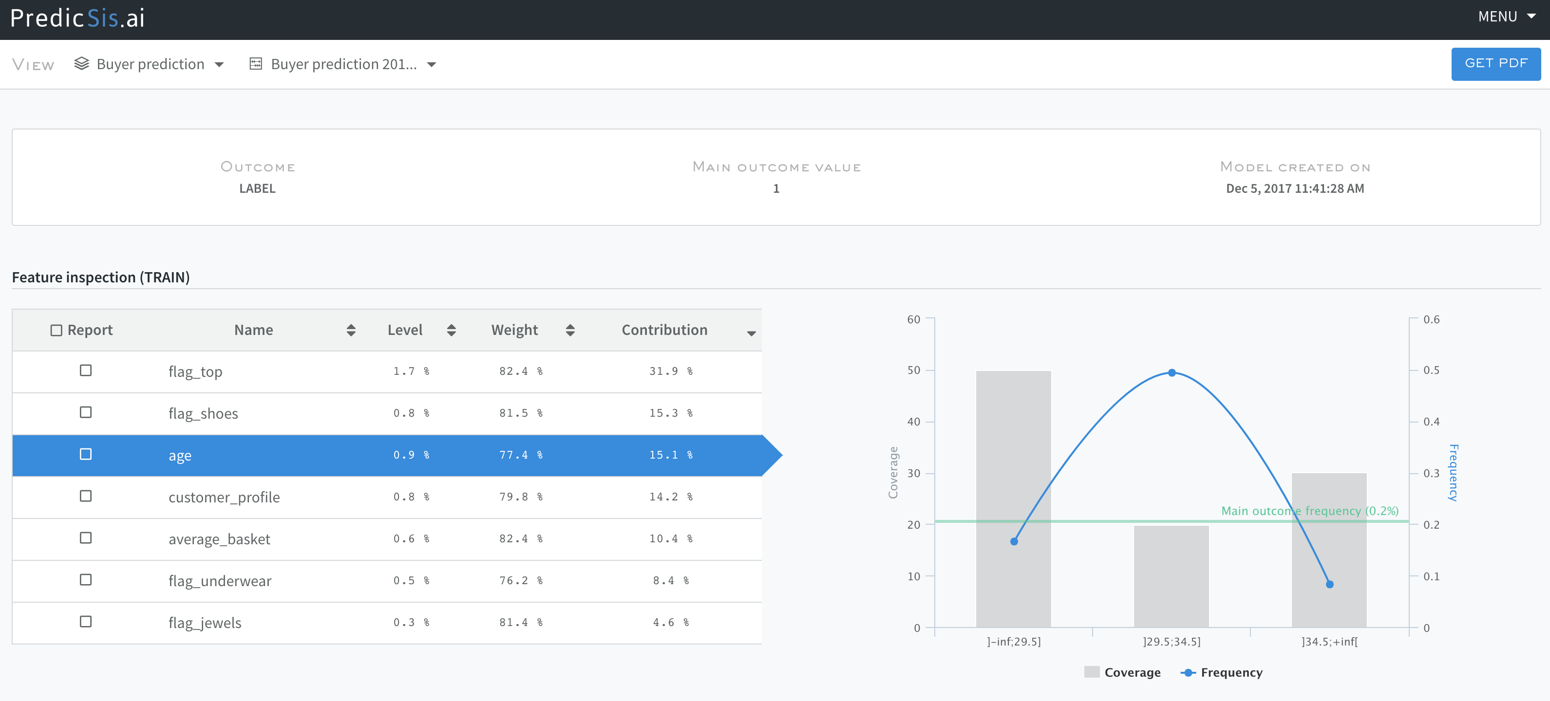
You are now ready to start working with the Predicsis.ai platform. First create a new project and upload all your data (Master, Orders, Emails and VisitedPages). The workflow is split between feature importance exploration followed by feature selection and data export. Start by exploring the Master file since it contains the outcome variable (LABEL). The following screenshot shows the relative importance of the different variables from that file. For instance, we see that the age variable contributes for 15% of the model prediction and is split in 3 bins each with a different coverage and frequency. This visualization gives us a good way to understand what really drives our predictions.
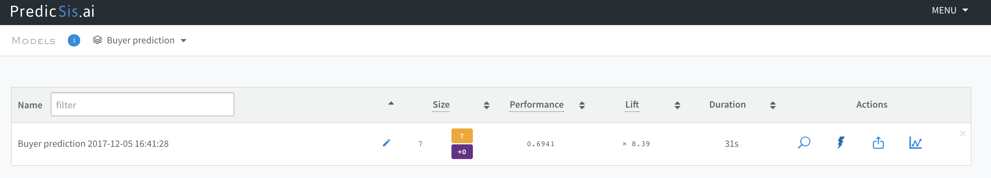
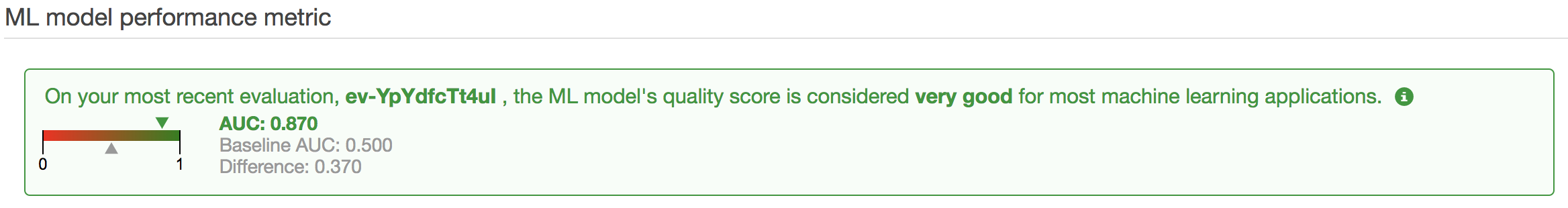
As shown in the next screenshot, our first model achieves a Gini score of 0.69 with Gini = 2 * AUC -1 where AUC is the classic Area Under Curve.
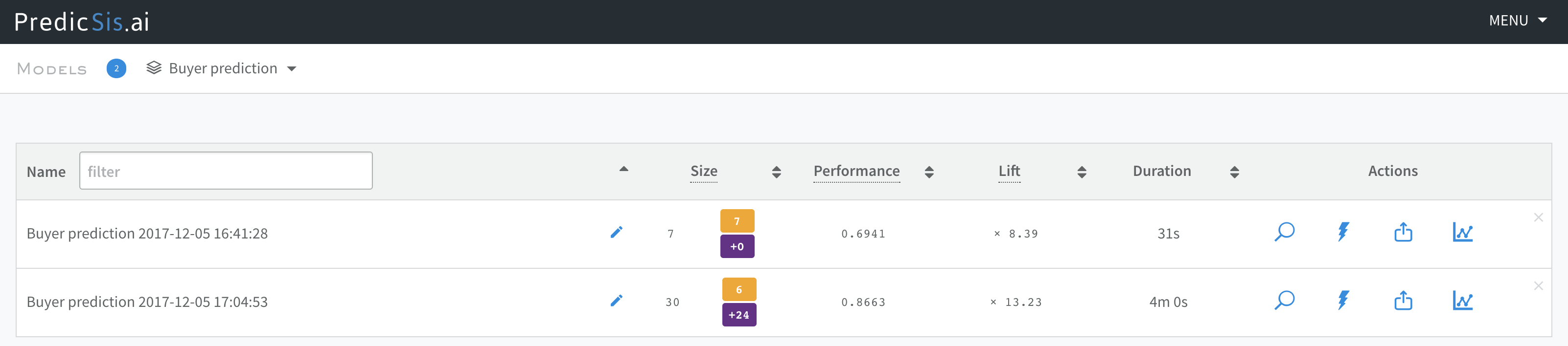
Now we can improve on that model by adding the data files to the feature mix.
In the next screenshot, we add the orders file and tell the model to generate 100 new feature aggregates and only keep a total of 30 features for our model. We explore the feature space and at the same time limit its dimension. Doing so will bring to the surface new features and create a new model with improved performances.
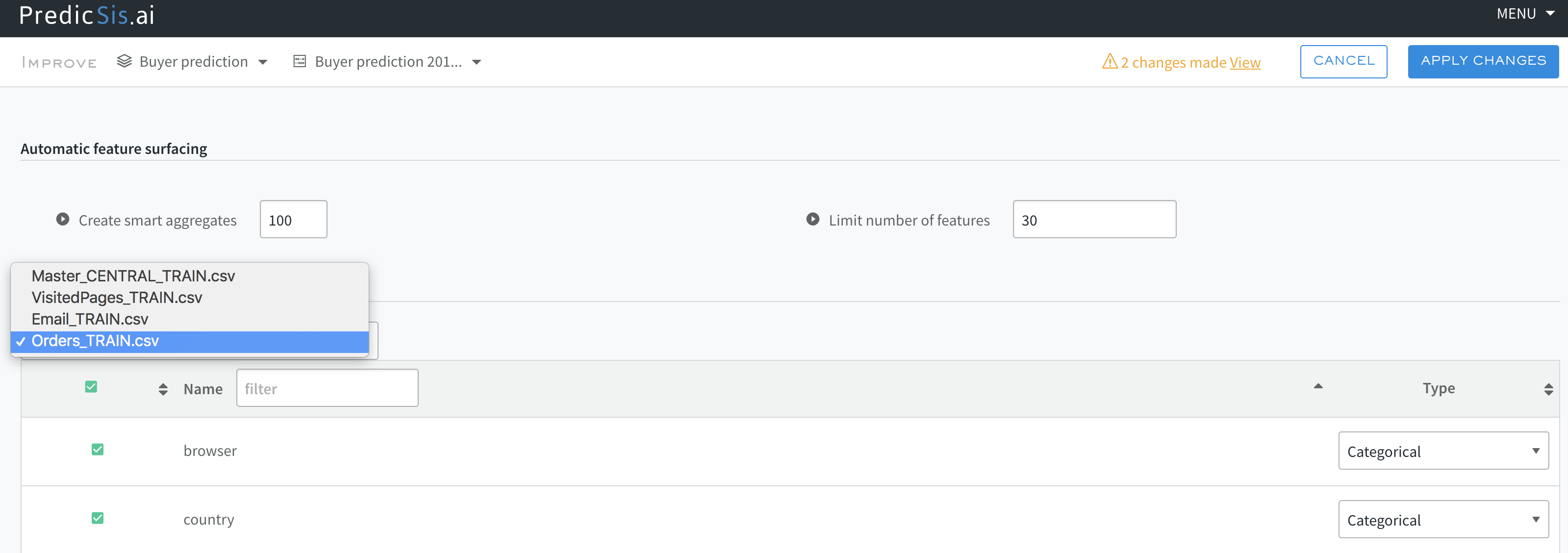
As we see below, our model’s performance has been sgnificantly improved from 0.69 to 0.87 while keeping the total number of features to 30: 6 of which come from the Master file, and 24 are new aggregates obtained from the order file.
We can iterate that feature generation process and add the other files (VisitedPages, Emails) to the feature mix, have the platform create and assess new aggregates and only keep the most important and powerful variables.
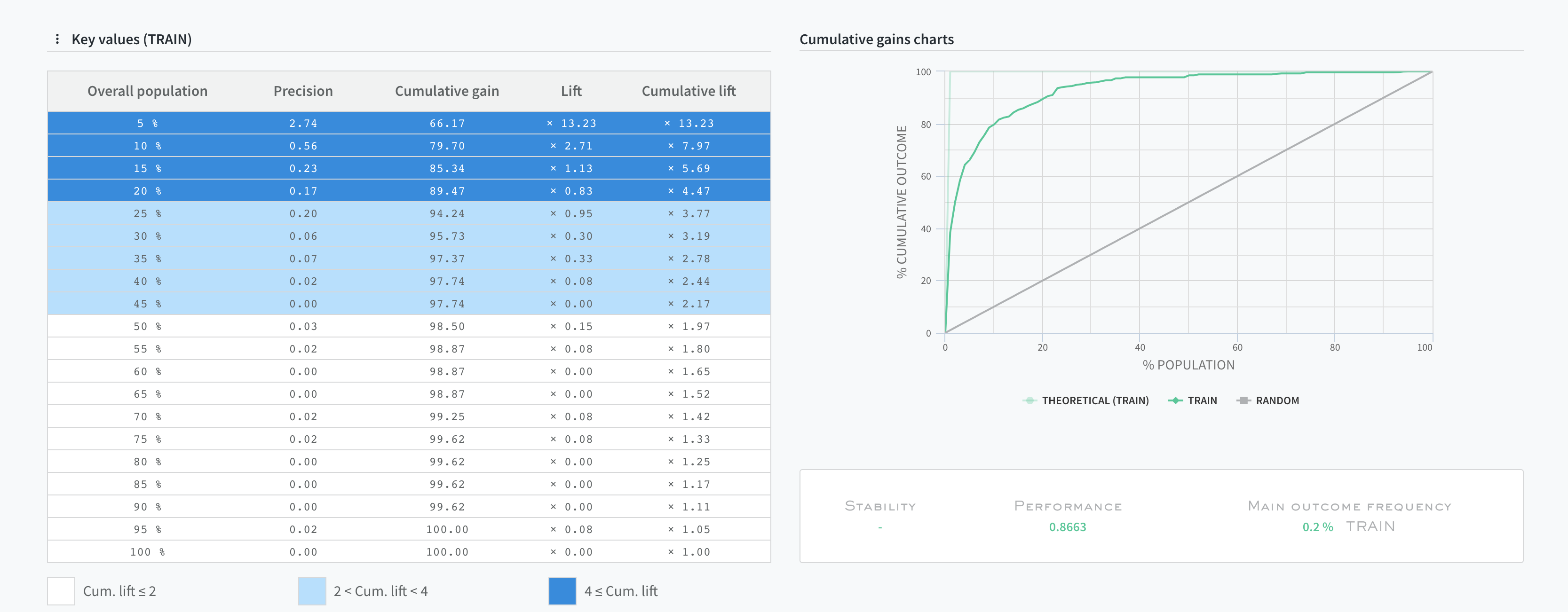
This is just a glimpse of Predicsis.ai capabilities. Predicsis.ai also offers rich visualizations to assess and understands the lift and cumulative gains related to the population slice.
Note that all these steps can also be carried out using the Predicsis.ai python SDK. The aggregation functions are quite simple (simple selects, binning or simple stats: mean, std, median). These functions can for the most part be implemented in SQL at the data extraction level directly from the database and therefore straightforward to apply on unseen production data. It’s also possible to use PredicSis.ai in batch mode to materialize those features on any new data with the same relational structure.
We can now export our optimized dataset to AWS ML and build a prediction model. To do so we follow the standard AWS ML workflow:
-
Upload the training data to S3
-
Define a data source. Let AWS ML infer the schema, double check and validate it.
-
Let AWS create the training and testing subsets.
-
AWS ML will suggest default transformations aka recipes which consists mostly in binning continuous variables. These binning transformations are important to achieve good predictions. You can either accept the suggested bins or the ones inferred by PredicSis.ai.
-
Train the model. With parameter tuning reduced to the bare minimum, you will only have to choose the type and strength of regularization
-
Wait a few minutes for the evaluation results.
-
if satisfied by the prediction score, create an end point with a click.
You now have a fully trained predictive model, based on a highly optimized features set, all in a matter of minutes without involving any scripting.
For that particular dataset, we obtain an AUC of 0.87 with the Predicsis.ai boosted dataset, which is very decent for such an imbalanced dataset so little efforts.
As predictive analytics becomes a must have for companies big and small, the need for fast and reliable data pipelines that can be easily understood and interpreted grows stronger. Using existing AWS based services available through simple UI we are able to build efficient end to end predictive models. From multi-relational raw data to optimized training datasets, powerful models and stable production end points. The reliability of this approach is grounded on the robust mathematical methods that these two services are built upon: Bayesian optimization for feature extraction and stochastic optimization for model training. Methods that have been studied for decades and that can be safely and simply exploited by business users for real life data projects.