We review the math and code needed to fit a Gaussian Process (GP) regressor to data. We conclude with a demo of a popular application, fast function minimization through GP-guided search. The gif below illustrates this approach in action — the red points are samples from the hidden red curve. Using these samples, we attempt to leverage GPs to find the curve’s minimum as fast as possible.
Appendices contain quick reviews on (i) the GP regressor posterior derivation, (ii) SKLearn’s GP implementation, and (iii) GP classifiers.
Follow us on twitter for new submission alerts!
Introduction
Gaussian Processes (GPs) provide a tool for treating the following general problem: A function $f(x)$ is sampled at $n$ points, resulting in a set of noisy$^1$ function measurements, ${f(x_i) = y_i \pm \sigma_i, i = 1, \ldots, n}$. Given these available samples, can we estimate the probability that $f = \hat{f}$, where $\hat{f}$ is some candidate function?
To decompose and isolate the ambiguity associated with the above challenge, we begin by applying Bayes’s rule,\begin{eqnarray} \label{Bayes} \tag{1}p(\hat{f} \vert {y}) = \frac{p({y} \vert \hat{f} ) p(\hat{f})}{p({y}) }.\end{eqnarray}The quantity at left above is shorthand for the probability we seek — the probability that $f = \hat{f}$, given our knowledge of the sampled function values ${y}$. To evaluate this, one can define and then evaluate the quantities at right. Defining the first in the numerator requires some assumption about the source of error in our measurement process. The second function in the numerator is the prior — it is here where the greatest assumptions must be taken. For example, we’ll see below that the prior effectively dictates the probability of a given smoothness for the $f$ function in question.
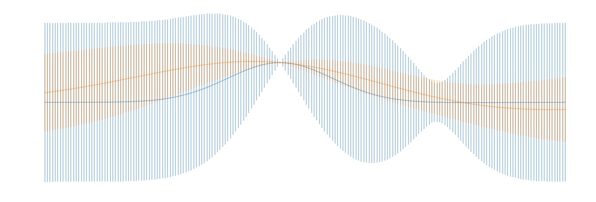
In the GP approach, both quantities in the numerator at right above are taken to be multivariate Normals / Gaussians. The specific parameters of this Gaussian can be selected to ensure that the resulting fit is good — but the Normality requirement is essential for the mathematics to work out. Taking this approach, we can write down the posterior analytically, which then allows for some useful applications. For example, we used this approach to obtain the curves shown in the top figure of this post — these were obtained through random sampling from the posterior of a fitted GP, pinned to equal measured values at the two pinched points shown. Posterior samples are useful for visualization and also for taking Monte Carlo averages.
In this post, we (i) review the math needed to calculate the posterior above, (ii) discuss numerical evaluations and fit some example data using GPs, and (iii) review how a fitted GP can help to quickly minimize a cost function — eg a machine learning cross-validation score. Appendices cover the derivation of the GP regressor posterior, SKLearn’s GP implementation, and GP Classifiers.
Our minimal python class SimpleGP used below is available on our GitHub, here.
Note: To understand the mathematical details covered in this post, one should be familiar with multivariate normal distributions — these are reviewed in our prior post, here. These details can be skipped by those primarily interested in applications.
Analytic evaluation of the posterior
To evaluate the left side of (\ref{Bayes}), we will evaluate the right. Only the terms in the numerator need to be considered, because the denominator does not depend on $\hat{f}$. This means that the denominator must equate to a normalization factor, common to all candidate functions. In this section, we will first write down the assumed forms for the two terms in the numerator and then consider the posterior that results.
The first assumption that we will make is that if the true function is $\hat{f}$, then our $y$-measurements are independent and Gaussian-distributed about $\hat{f}(x)$. This assumption implies that the first term on the right of (\ref{Bayes}) is\begin{eqnarray} \tag{2} \label{prob}p({y} \vert \hat{f} ) \equiv \prod_{i=1}^n \frac{1}{\sqrt{2 \pi \sigma_i^2}} \exp \left ( – \frac{(y_i – \hat{f}(x_i) )^2}{2 \sigma_i^2} \right).\end{eqnarray}The $y_i$ above are the actual measurements made at our sample points, and the $\sigma_i^2$ are their variance uncertainties.
The second thing we must do is assume a form for $p(\hat{f})$, our prior. We restrict attention to a set of points ${x_i: i = 1, \ldots, N}$, where the first $n$ points are the points that have been sampled, and the remaining $(N-n)$ are test points at other locations — points where we would like to estimate the joint statistics$^2$ of $f$. To progress, we simply assume a multi-variate Normal distribution for $f$ at these points, governed by a covariance matrix $\Sigma$. This gives\begin{eqnarray} \label{prior} \tag{3}&&p(f(x_1), \ldots, f(x_N) ) \sim \&& \frac{1}{\sqrt{ (2 \pi)^{N} \vert \Sigma \vert }} \exp \left ( – \frac{1}{2} \sum_{ij=1}^N f_i \Sigma^{-1}_{ij} f_j \right).\end{eqnarray}Here, we have introduced the shorthand, $f_i \equiv f(x_i)$. Notice that we have implicitly assumed that the mean of our normal distribution is zero above. This is done for simplicity: If a non-zero mean is appropriate, this can be added in to the analysis, or subtracted from the underlying $f$ to obtain a new one with zero mean.
The particular form of $\Sigma$ is where all of the modeler’s insight and ingenuity must be placed when working with GPs. Researchers who know their topic very well can assert well-motivated, complex priors — often taking the form of a sum of terms, each capturing some physically-relevant contribution to the statistics of their problem at hand. In this post, we’ll assume the simple form\begin{eqnarray} \tag{4} \label{covariance}\Sigma_{ij} \equiv \sigma^2 \exp \left( – \frac{(x_i – x_j)^2}{2 l^2}\right).\end{eqnarray}Notice that with this assumed form, if $x_i$ and $x_j$ are close together, the exponential will be nearly equal to one. This ensures that nearby points are highly correlated, forcing all high-probability functions to be smooth. The rate at which (\ref{covariance}) dies down as two test points move away from each another is controlled by the length-scale parameter $l.$ If this is large (small), the curve will be smooth over a long (short) distance. We illustrate these points in the next section, and also explain how an appropriate length scale can be inferred from the sample data at hand in the section after that.
Now, if we combine (\ref{prob}) and (\ref{prior}) and plug this into (\ref{Bayes}), we obtain an expression for the posterior, $p(f \vert {y})$. This function is an exponential whose argument is a quadratic in the $f_i$. In other words, like the prior, the posterior is a multi-variate normal. With a little work, one can derive explicit expressions for the mean and covariance of this distribution: Using block notation, with $0$ corresponding to the sample points and $1$ to the test points, the marginal distribution at the test points is\begin{eqnarray} \tag{5} \label{posterior}&& p(\textbf{f}1 \vert {y}) =\&& N\left ( \Sigma{10} \frac{1}{\sigma^2 I_{00} + \Sigma_{00}} \cdot \textbf{y}, \Sigma_{11} – \Sigma_{10} \frac{1}{\sigma^2 I_{00} + \Sigma_{00}} \Sigma_{01} \right).\end{eqnarray}Here,\begin{eqnarray} \tag{6} \label{sigma_mat}\sigma^2 I_{00} \equiv\left( \begin{array}{cccc}\sigma_1^2 & 0 & \ldots &0 \0 & \sigma_2^2 & \ldots &0 \\ldots & & & \0 & 0 & \ldots & \sigma_n^2\end{array} \right),\end{eqnarray}and $\textbf{y}$ is the length-$n$ vector of measurements,\begin{eqnarray}\tag{7} \label{y_vec}\textbf{y}^T \equiv (y_1, \ldots, y_n).\end{eqnarray}
Equation (\ref{posterior}) is one of the main results for Gaussian Process regressors — this result is all one needs to evaluate the posterior. Notice that the mean at all points is linear in the sampled values $\textbf{y}$ and that the variance at each point is reduced near the measured values. Those interested in a careful derivation of this result can consult our appendix — we actually provide two derivations there. However, in the remainder of the body of the post, we will simply explore applications of this formula.
Numerical evaluations of the posterior
In this section, we will demonstrate how two typical applications of (\ref{posterior}) can be carried out: (i) Evaluation of the mean and standard deviation of the posterior distribution at a test point $x$, and (ii) Sampling functions $\hat{f}$ directly from the posterior. The former is useful in that it can be used to obtain confidence intervals for $f$ at all locations, and the latter is useful both for visualization and also for obtaining general Monte Carlo averages over the posterior. Both concepts are illustrated in the header image for this post: In this picture, we fit a GP to a one-d function that had been measured at two locations. The blue shaded region represents a one-sigma confidence interval for the function value at each location, and the colored curves are posterior samples.
The code for our SimpleGP fitter class is available on our GitHub. We’ll explain a bit how this works below, but those interested in the details should examine the code — it’s a short script and should be largely self-explanatory.
Intervals
The code snippet below initializes our SimpleGP class, defines some sample locations, values, and uncertainties, then evaluates the mean and standard deviation of the posterior at a set of test points. Briefly, this carried out as follows: The fit method evaluates the inverse matrix $\left [ \sigma^2 I_{00} + \Sigma_{00} \right]^{-1}$ that appears in (\ref{posterior}) and saves the result for later use — this allows us to avoid reevaluation of this inverse at each test point. Next, (\ref{posterior}) is evaluated once for each test point through the call to the interval method.
In the above, WIDTH_SCALE and LENGTH_SCALE are needed to specify the covariance matrix (\ref{covariance}). The former corresponds to $\sigma$ and the latter to $l$ in that equation. Increasing WIDTH_SCALE corresponds to asserting less certainty as to the magnitude of unknown function and increasing LENGTH_SCALE corresponds to increasing how smooth we expect the function to be. The figure below illustrates these points: Here, the blue intervals were obtained by setting WIDTH_SCALE = LENGTH_SCALE = 1 and the orange intervals were obtained by setting WIDTH_SCALE = 0.5 and LENGTH_SCALE = 2. The result is that the orange posterior estimate is tighter and smoother than the blue posterior. In both plots, the solid curve is a plot of the mean of the posterior distribution, and the vertical bars are one sigma confidence intervals.
Posterior samples
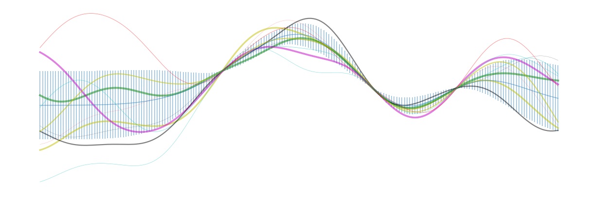
To sample actual functions from the posterior, we will simply evaluate the mean and covariance matrix in (\ref{posterior}) again, this time passing in the multiple test point locations at which we would like to know the resulting sampled functions. Once we have the mean and covariance matrix of the posterior at these test points, we can pull samples from (\ref{posterior}) using an external library for multivariate normal sampling — for this purpose, we used the python package numpy. The last step in the code snippet below carries out these steps.
Notice that in lines 2-4 here, we’ve added in a few additional function sample locations (for fun). The resulting intervals and posterior samples are shown in the figure below. Notice that near the sampled points, the posterior is fairly well localized. However, on the left side of the plot, the posterior approaches the prior once we have moved a distance $\geq 1$, the length scale chosen for the covariance matrix (\ref{covariance}).
Selecting the covariance hyper-parameters
In the above, we demonstrated that the length scale of our covariance form dramatically affects the posterior — the shape of the intervals and also of the samples from the posterior. Appropriately setting these parameters is a general problem that can make working with GPs a challenge. Here, we describe two methods that can be used to intelligently set such hyper-parameters, given some sampled data.
Cross-validation
A standard method for setting hyper-parameters is to make use of a cross-validation scheme. This entails splitting the available sample data into a training set and a test set. One fits the GP to the training set using one set of hyper-parameters, then evaluates the accuracy of the model on the held out test set. One then repeats this process across many hyper-parameter choices, and selects that set which resulted in the best test set performance.
Marginal Likelihood Maximization
Often, one is interested in applying GPs in limits where evaluation of samples is expensive. This means that one often works with GPs in limits where only a small number of samples are available. In cases like this, the optimal hyper-parameters can vary quickly as the number of training points is increased. This means that the optimal selections obtained from a cross-validation schema may be far from the optimal set that applies when one trains on the full sample set$^3$.
An alternative general approach for setting the hyper-parameters is to maximize the marginal likelihood. That is, we try to maximize the likelihood of seeing the samples we have seen — optimizing over the choice of available hyper-parameters. Formally, the marginal likelihood is evaluated by integrating out the unknown $\hat{f}^4$,\begin{eqnarray} \tag{8}p({y} \vert \Sigma) \equiv \int p({y} \vert f) p(f \vert \Sigma) df.\end{eqnarray}Carrying out the integral directly can be done just as we have evaluated the posterior distribution in our appendix. However, a faster method is to note that after integrating out the $f$, the $y$ values must be normally distributed as\begin{eqnarray}\tag{9}p({y} \vert \Sigma) \sim N(0, \Sigma + \sigma^2 I_{00}),\end{eqnarray}where $\sigma^2 I_{00}$ is defined as in (\ref{sigma_mat}). This gives\begin{eqnarray} \tag{10} \label{marginallikelihood}\log p({y}) \sim – \log \vert \Sigma + \sigma^2 I_{00} \vert – \textbf{y} \cdot ( \Sigma + \sigma^2 I_{00} )^{-1} \cdot \textbf{y}.\end{eqnarray}The two terms above compete: The second term is reduced by finding the covariance matrix that maximizes the exponent. Maximizing this alone would tend to result in an overfitting of the data. However, this term is counteracted by the first, which is the normalization for a Gaussian integral. This term becomes larger given short decay lengths and low diagonal variances. It acts as regularization term that suppresses overly complex fits.
In practice, to maximize (\ref{marginallikelihood}), one typically makes use of gradient descent, using analytical expressions for the gradient. This is the approach taken by SKLearn. Being able to optimize the hyper-parameters of a GP is one of this model’s virtures. Unfortunately, (\ref{marginallikelihood}) is not guaranteed to be convex and multiple local minima often exist. To obtain a good minimum, one can attempt to initialize at some well-motivated point. Alternatively, one can reinitialize the gradient descent repeatedly at random points, finally selecting the best option at the end.
Function minimum search and machine learning
We’re now ready to introduce one of the popular application of GPs: fast, guided function minimum search. In this problem, one is able to iteratively obtain noisy samples of a function, and the aim is to identify as quickly as possible the global minimum of the function. Gradient descent could be applied in cases like this, but this approach generally requires repeated sampling if the function is not convex. To reduce the number of steps / samples required, one can attempt to apply a more general, explore-exploit type strategy — one balancing the desire to optimize about the current best known minimum with the goal of seeking out new local minima that are potentially even better. GP posteriors provide a natural starting point for developing such strategies.
The idea behind the GP-guided search approach is to develop a score function on top of the GP posterior. This score function should be chosen to encode some opinion of the value of searching a given point — preferably one that takes an explore-exploit flavor. Once each point is scored, the point with the largest (or smallest, as appropriate) score is sampled. The process is then repeated iteratively until one is satisfied. Many score functions are possible. We discuss four possible choices below, then give an example.
- Gaussian Lower Confidence Bound (GLCB).The GLCB scores each point $x$ as\begin{eqnarray}\tag{11}s_{\kappa}(x) = \mu(x) – \kappa \sigma(x).\end{eqnarray}Here, $\mu$ and $\sigma$ are the GP posterior estimates for the mean and standard deviation for the function at $x$ and $\kappa$ is a control parameter. Notice that the first $\mu(x)$ term encourages exploitation around the best known local minimum. Similarly, the second $\kappa \sigma$ term encourages exploration — search at points where the GP is currently most unsure of the true function value.