Ensemble learning methods are widely used nowadays for its predictive performance improvement. Ensemble learning combines multiple predictions (forecasts) from one or multiple methods to overcome accuracy of simple prediction and to avoid possible overfit. In the domain of time series forecasting, we have somehow obstructed situation because of dynamic changes in coming data. However, when a single regression model is used for forecasting, time dependency is not the obstacle, we can tune it at current time of a sliding window. For this reason, in this post, I will describe you two simple ensemble learning methods - Bagging and Random Forest. Bagging will be used with combination of two simple regression trees methods used in the previous post (RPART and CTREE). I will not repeat most of the things mentioned there so check it first if you didn’t make it already: Using regression trees for forecasting double-seasonal time series with trend.

You will learn in this post how to:

tune simple regression trees methods by Bagging
set important hyperparameters of decision tree methods and randomized them in Bagging
use Random Forest method for forecasting time series
set hyperparameters of Random Forest and find it optimally by grid search method

Time series data of electricity consumption

As in previous posts, I will use smart meter data of electricity consumption for demonstrating forecasting of seasonal time series. The dataset of aggregated electricity load of consumers from an anonymous area is used. Time series data have the length of 17 weeks.

Firstly, let’s scan all of the needed packages for data analysis, modeling and visualizing.

library(feather) # data import
library(data.table) # data handle
library(rpart) # decision tree method
library(party) # decision tree method
library(forecast) # forecasting methods
library(randomForest) # ensemble learning method
library(ggplot2) # visualizations

Now read the mentioned time series data by read_feather to one data.table. The dataset can be found on my github repo, the name of the file is DT_load_17weeks.

DT <- as.data.table(read_feather(“DT_load_17weeks”))

And store information of the date and period of time series that is 48.

n_date <- unique(DT[, date]) period <- 48

For data visualization needs, store my favorite ggplot theme settings by function `theme`.

theme_ts <- theme(panel.border = element_rect(fill = NA, colour = “grey10”), panel.background = element_blank(), panel.grid.minor = element_line(colour = “grey85”), panel.grid.major = element_line(colour = “grey85”), panel.grid.major.x = element_line(colour = “grey85”), axis.text = element_text(size = 13, face = “bold”), axis.title = element_text(size = 15, face = “bold”), plot.title = element_text(size = 16, face = “bold”), strip.text = element_text(size = 16, face = “bold”), strip.background = element_rect(colour = “black”), legend.text = element_text(size = 15), legend.title = element_text(size = 16, face = “bold”), legend.background = element_rect(fill = “white”), legend.key = element_rect(fill = “white”))

I will use three weeks of data of electricity consumption for training regression trees methods. Forecasts will be performed to one day ahead. Let’s extract train and test set from the dataset.

data_train <- DT[date %in% n_date[1:21]] data_test <- DT[date %in% n_date[22]]

And visualize the train part:

ggplot(data_train, aes(date_time, value)) + geom_line() + labs(x = “Date”, y = “Load (kW)”) + theme_ts

![](https://petolau.github.io/images/post_6/unnamed-chunk-7-1.png)

## Bagging

**Bagging** or bootstrap aggregating, is ensemble learning meta-algorithm used to improve prediction accuracy and to overcome (avoid) overfitting. The algorithm is very simple. The first step is sampling a training dataset with replacement with some defined sample ratio (e.g. 0.7). Then a model is trained on a new train set. This procedure is repeated *N_boot* times (e.g. 100). Final ensemble prediction is just average of *N_boot* predictions. For aggregating predictions, the median can be also used and will be used in this post.

### Bagging + RPART

The first “bagged” method is RPART (CART) tree. Training set consists of lagged electricity load by one day and double-seasonal Fourier terms (daily and weekly seasonality). Electricity consumption is firstly detrended by STL decomposition and trend part is forecasted (modeled) by ARIMA (`auto.arima` function). Seasonal and remainder part is then forecasted by regression tree model. More detailed description and explanations are in my previous post about regression trees methods. Let’s define train and test data (by `matrix_train` and `matrix_test`).

data_ts <- ts(data_train$value, freq = period * 7) decomp_ts <- stl(data_ts, s.window = “periodic”, robust = TRUE)$time.series trend_part <- ts(decomp_ts[,2])

trend_fit <- auto.arima(trend_part) # ARIMA trend_for <- as.vector(forecast(trend_fit, period)$mean) # trend forecast data_msts <- msts(data_train$value, seasonal.periods = c(period, period*7))

K <- 2 fuur <- fourier(data_msts, K = c(K, K)) # Fourier features to model (Daily and Weekly)

N <- nrow(data_train) window <- (N / period) - 1

new_load <- rowSums(decomp_ts[, c(1,3)]) # detrended original time series lag_seas <- decomp_ts[1:(period*window), 1] # lag feature to model

matrix_train <- data.table(Load = tail(new_load, window*period), fuur[(period + 1):N,], Lag = lag_seas)

create testing data matrix

test_lag <- decomp_ts[((period*window)+1):N, 1] fuur_test <- fourier(data_msts, K = c(K, K), h = period)

matrix_test <- data.table(fuur_test, Lag = test_lag)

I will perform 100 bootstrapped forecasts by RPART, that will be stored in the matrix of size \( 100\times 48 \) (`pred_mat`). Additional four parameters will be also sampled (randomized) to avoid overfitting. Sample ratio for sampling train set is sampled in the range from 0.7 to 0.9. Three hyperparameters of RPART are sampled also: `minsplit`, `maxdepth` and complexity parameter `cp`. Hyperparameters are sampled around values set on my previous post modeling.

N_boot <- 100 # number of bootstraps

pred_mat <- matrix(0, nrow = N_boot, ncol = period) for(i in 1:N_boot) {

matrixSam <- matrix_train[sample(1:(N-period), floor((N-period) * sample(seq(0.7, 0.9, by = 0.01), 1)), replace = TRUE)] # sampling with sampled ratio from 0.7 to 0.9 tree_bag <- rpart(Load ~ ., data = matrixSam, control = rpart.control(minsplit = sample(2:3, 1), maxdepth = sample(26:30, 1), cp = sample(seq(0.0000009, 0.00001, by = 0.0000001), 1)))

# new data and prediction pred_mat[i,] <- predict(tree_bag, matrix_test) + mean(trend_for) }

Let’s compute median of forecasts and visualize all created forecasts. For `ggplot` visualization needs we must use `melt` function to the matrix of forecasts `pred_mat`.

pred_melt_rpart <- data.table(melt(pred_mat))

pred_ave_rpart <- pred_melt_rpart[, .(value = median(value)), by = .(Var2)] pred_ave_rpart[, Var1 := “RPART_Bagg”]

ggplot(pred_melt_rpart, aes(Var2, value, group = Var1)) + geom_line(alpha = 0.75) + geom_line(data = pred_ave_rpart, aes(Var2, value), color = “firebrick2”, alpha = 0.9, size = 2) + labs(x = “Time”, y = “Load (kW)”, title = “Bagging with RPART”) + theme_ts

![](https://petolau.github.io/images/post_6/unnamed-chunk-11-1.png)

The red line is median of forecasts. We can see that created forecasts by RPART have typical rectangular shape, but final ensemble forecasts has nice smooth behaviour. For comparison, compute forecast by RPART on whole train set and compare it with previous results. I am using function `RpartTrend` from my previous post.

simple_rpart <- RpartTrend(DT, n_date[1:21], K = 2) pred_rpart <- data.table(value = simple_rpart, Var2 = 1:48, Var1 = “RPART”)

ggplot(pred_melt_rpart, aes(Var2, value, group = Var1)) + geom_line(alpha = 0.75) + geom_line(data = pred_ave_rpart, aes(Var2, value), color = “firebrick2”, alpha = 0.8, size = 1.8) + geom_line(data = pred_rpart, aes(Var2, value), color = “dodgerblue2”, alpha = 0.8, size = 1.8) + labs(x = “Time”, y = “Load (kW)”, title = “Bagging with RPART and comparison with simple RPART”) + theme_ts

![](https://petolau.github.io/images/post_6/unnamed-chunk-12-1.png)

The blue line is simple RPART forecast. The difference between ensemble forecast and simple one is not very evident in this scenario.

## Bagging with CTREE

The second “bagged” regression tree method is CTREE. I will randomize only `mincriterion` hyperparameter of CTREE method that decisions about splitting a node. The sample ratio is of course sampled (randomized) as well as in the previous case with RPART.

pred_mat <- matrix(0, nrow = N_boot, ncol = period) for(i in 1:N_boot) {

matrixSam <- matrix_train[sample(1:(N-period), floor((N-period) * sample(seq(0.7, 0.9, by = 0.01), 1)), replace = TRUE)] # sampling with sampled ratio from 0.7 to 0.9 tree_bag <- party::ctree(Load ~ ., data = matrixSam, controls = party::ctree_control(teststat = c(“quad”), testtype = c(“Teststatistic”), mincriterion = sample(seq(0.88, 0.97, by = 0.005), 1), minsplit = 1, minbucket = 1, mtry = 0, maxdepth = 0))

# new data and prediction pred_mat[i,] <- predict(tree_bag, matrix_test) + mean(trend_for) }

Let’s visualize results:

pred_melt_ctree <- data.table(melt(pred_mat))

pred_ave_ctree <- pred_melt_ctree[, .(value = median(value)), by = .(Var2)] pred_ave_ctree[, Var1 := “CTREE_Bagg”]

ggplot(pred_melt_ctree, aes(Var2, value, group = Var1)) + geom_line(alpha = 0.75) + geom_line(data = pred_ave_ctree, aes(Var2, value), color = “firebrick2”, alpha = 0.9, size = 2) + labs(x = “Time”, y = “Load (kW)”, title = “Bagging with CTREE”) + theme_ts

![](https://petolau.github.io/images/post_6/unnamed-chunk-14-1.png)

Again, behaviour of bootstrapped forecasts is very rectangular and the final ensemble forecast is much more smoother. Compare it also with forecast performed on whole train set. I am using function `CtreeTrend` from my previous post.

simple_ctree <- CtreeTrend(DT, n_date[1:21], K = 2) pred_ctree <- data.table(value = simple_ctree, Var2 = 1:48, Var1 = “CTREE”)

ggplot(pred_melt_ctree, aes(Var2, value, group = Var1)) + geom_line(alpha = 0.75) + geom_line(data = pred_ave_ctree, aes(Var2, value), color = “firebrick2”, alpha = 0.8, size = 1.8) + geom_line(data = pred_ctree, aes(Var2, value), color = “dodgerblue2”, alpha = 0.8, size = 1.8) + labs(x = “Time”, y = “Load (kW)”, title = “Bagging with CTREE and comparison with simple CTREE”) + theme_ts

![](https://petolau.github.io/images/post_6/unnamed-chunk-15-1.png)

The simple forecast is a little bit more rectangular than ensemble one.

## Random Forest

**Random Forest** is an improvement of Bagging ensemble learning method. It uses a modified tree learning algorithm that selects, at each candidate split in the learning process, a random subset of the features. This process is sometimes called “feature bagging”. The classical Bagging is also used in the method of course. Hyperparameters of Random Forest is similar to those in RPART method. Additional ones are: number of trees (`ntree`); number of variables sampled in each candidate split (`mtry`). Importance of variables can be also incorporated to learning process in order to enhance the performance. Random Forest is implemented in **R** by package `randomForest` and same-named function. Default settings for hyperparameters are: `mtry` = p/3 (where p is number of features), so 9/3 = 3 in our case, and `nodesize` = 5. I will set a number of trees to 1000.

rf_model <- randomForest(Load ~ ., data = data.frame(matrix_train), ntree = 1000, mtry = 3, nodesize = 5, importance = TRUE)

Whereas we use ensemble of CART trees in Random Forest, we can compute variable importance. Checking variable importance can be important for extracting just most valuable features and to analyze dependencies and correlations in data. Let’s check variable importance by `varImpPlot`.

varImpPlot(rf_model, main = "Variable importance")

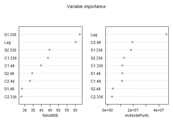
We can see that Lag and S1.336 (weekly seasonal feature in sinus form) features have best scores in both measures. It implies that weekly seasonality and and lagged values of load are most important for our training data.

Let’s compute also forecast.

pred_rf <- predict(rf_model, data.frame(matrix_test)) + mean(trend_for)

And compare forecasts from all ensemble learning approaches so far and real electricity load.

pred_rf <- data.table(value = pred_rf, Var2 = 1:48, Var1 = “RF”)

pred_true <- data.table(value = data_test$value, Var2 = 1:48, Var1 = “Real”) preds_all <- rbindlist(list(pred_ave_rpart, pred_ave_ctree, pred_rf, pred_true), use.names = T)

ggplot(preds_all, aes(Var2, value, color = as.factor(Var1))) + geom_line(alpha = 0.7, size = 1.2) + labs(x = “Time”, y = “Load (kW)”, title = “Comparison of Ensemble Learning forecasts”) + guides(color=guide_legend(title=”Method”)) + theme_ts

![](https://petolau.github.io/images/post_6/unnamed-chunk-19-1.png)

There are just small differences.

## Hyperparameters tuning - grid search

It is always highly recommended to tune hyperparameters of our used method. By hyperparameters tuning, we can significantly improve predictive performance. I will try to tune two hyperparameters of **Random Forest**, `mtry` and `nodesize`, by **grid search** method.
For specificity of time series forecasting, I proposed my own function of grid search (`gridSearch`). The evaluation is based on sliding window forecasting, so forecasting error is average of errors in some range of time. I also created my own Random Forest function (`RFgrid`) that is compatible with grid search function. The output of `gridSearch` function is matrix of average MAPE (Mean Absolute Percentage Error) values corresponding to hyperparameters used.

RFgrid <- function(data_train, param1, param2, K, period = 48) {

N <- length(data_train) window <- (N / period) - 1 data_ts <- msts(data_train, seasonal.periods = c(period, period*7))

fuur <- fourier(data_ts, K = c(K, K)) fuur_test <- as.data.frame(fourier(data_ts, K = c(K, K), h = period))

data_ts <- ts(data_train, freq = period*7) decomp_ts <- stl(data_ts, s.window = “periodic”, robust = TRUE) new_load <- rowSums(decomp_ts$time.series[, c(1,3)]) trend_part <- ts(decomp_ts$time.series[,2])

trend_fit <- auto.arima(trend_part) trend_for <- as.vector(forecast(trend_fit, period)$mean) lag_seas <- decomp_ts$time.series[1:(period*window), 1]

matrix_train <- data.frame(Load = tail(new_load, window*period), fuur[(period+1):N,], Lag = lag_seas)

tree_2 <- randomForest(Load ~ ., data = matrix_train, ntree = 1000, mtry = param1, nodesize = param2, importance = TRUE) test_lag <- decomp_ts$time.series[((period*(window))+1):N, 1]

matrix_test <- data.frame(fuur_test, Lag = test_lag) pred_tree <- predict(tree_2, matrix_test) + mean(trend_for)

return(as.vector(pred_tree)) }

mape <- function(real, pred){ return(100 * mean(abs((real - pred)/real))) # MAPE - Mean Absolute Percentage Error } gridSearch <- function(Y, train.win = 21, FUN, param1, param2, period = 48) {

days <- length(Y)/period test.days <- days - train.win mape.matrix <- matrix(0, nrow = length(param1), ncol = length(param2)) row.names(mape.matrix) <- param1 colnames(mape.matrix) <- param2 forecast.rf <- vector(length = test.days*period)

for(i in seq_along(param1)){ for(j in seq_along(param2)){ for(k in 0:(test.days-1)){ train.set <- Y[((kperiod)+1):((periodk)+(train.winperiod))] forecast.rf[((kperiod)+1):((k+1)period)] <- FUN(train.set, param1 = param1[i], param2 = param2[j], K = 2) mape.matrix[i,j] <- mape(Y[-(1:(train.winperiod))], forecast.rf) } } return(mape.matrix) }

For our purpose, I will make 20 forecasts for each hyperparameter combination. I will test `nodesize` and `mtry` parameters for values \( 2,3,4,5,6 \). It is taking some time to compute, so be aware.

all_data <- DT$value[1:(period*41)] res_1 <- gridSearch(all_data, FUN = RFgrid, param1 = c(2,3,4,5,6), param2 = c(2,3,4,5,6))

Let’s check the results.

res_1

2 3 4 5 6

2 2.937151 2.931990 2.952967 2.970451 2.972355

3 2.888450 2.896477 2.897801 2.912977 2.914294

4 2.874241 2.878923 2.880959 2.882959 2.896501

5 2.876503 2.872179 2.873983 2.875953 2.882657

6 2.868838 2.872933 2.874093 2.867840 2.881881

And find the minimum.

c(mtry = row.names(res_1)[which(res_1 == min(res_1), arr.ind = TRUE)[1]], nodesize = colnames(res_1)[which(res_1 == min(res_1), arr.ind = TRUE)[2]])

## mtry nodesize 
## "6" "5"

So best (optimal) setting is mtry = 6 and nodesize = 5.

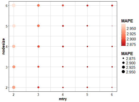
For better imagination and analysis of results, let’s visualize the computed grid of MAPE values.

data_grid <- data.table(melt(res_1))
colnames(data_grid) <- c("mtry", "nodesize", "MAPE")
 
ggplot(data_grid, aes(mtry, nodesize, size = MAPE, color = MAPE)) +
 geom_point() +
 scale_color_distiller(palette = "Reds") +
 theme_ts

We can see that lowest average MAPEs are for mtry = 6 and nodesize = 2 or 5.

Comparison

For more exact evaluation, I made comparison of five methods - simple RPART, simple CTREE, Bagging + RPART, Bagging + CTREE and Random Forest on whole available dataset (so 98 forecasts were performed). I created plotly boxplots graph of MAPE values from these 5 methods. Whole evaluation can be seen in the script that is stored in my GitHub repository.

We can see that Bagging really helps decrease forecasting error for RPART and CTREE. The Random Forest has best results among all tested methods, so I proposed suitable approach for seasonal time series forecasting.

Conclusion

In this post, I showed you how to use basic ensemble learning methods to improve forecasting accuracy. I used classical Bagging in combination with regression tree methods - RPART and CTREE. The extension of Bagging, Random Forest, was also used and evaluated. I showed you how to set important hyperparameters and how to tune them by grid search method. The Random Forest method comes most accurate and I highly recommend it for time series forecasting. But, it must be said that feature engineering is very important part also of regression modeling of time series. So, I don’t generalize results for every possible task of time series forecasting.

In the future post, I will write about other bootstrapping techniques for time series or Boosting.

Ensemble learning for time series forecasting in R

未知