We review binary logistic regression. In particular, we derive a) the equations needed to fit the algorithm via gradient descent, b) the maximum likelihood fit’s asymptotic coefficient covariance matrix, and c) expressions for model test point class membership probability confidence intervals. We also provide python code implementing a minimal “LogisticRegressionWithError” class whose “predict_proba” method returns prediction confidence intervals alongside its point estimates.
Our python code can be downloaded from our github page, here. Its use requires the jupyter, numpy, sklearn, and matplotlib packages.
Follow us on twitter for new submission alerts!
Introduction
The logistic regression model is a linear classification model that can be used to fit binary data — data where the label one wishes to predict can take on one of two values — e.g., $0$ or $1$. Its linear form makes it a convenient choice of model for fits that are required to be interpretable. Another of its virtues is that it can — with relative ease — be set up to return both point estimates and also confidence intervals for test point class membership probabilities. The availability of confidence intervals allows one to flag test points where the model prediction is not precise, which can be useful for some applications — eg fraud detection.
In this note, we derive the expressions needed to fit the logistic model to a training data set. We assume the training data consists of a set of $n$ feature vector- label pairs, ${(\vec{x}_i, y_i)$, for $i = 1, 2, \ldots, n}$, where the feature vectors $\vec{x}_i$ belong to some $m$-dimensional space and the labels are binary, $y_i \in {0, 1}.$ The logistic model states that the probability of belonging to class $1$ is given by\begin{eqnarray}\tag{1} \label{model1}p(y=1 \vert \vec{x}) \equiv \frac{1}{1 + e^{- \vec{\beta} \cdot \vec{x} } },\end{eqnarray}where $\vec{\beta}$ is a coefficient vector characterizing the model. Note that with this choice of sign in the exponent, predictor vectors $\vec{x}$ having a large, positive component along $\vec{\beta}$ will be predicted to have a large probability of being in class $1$. The probability of class $0$ is given by the complement,\begin{eqnarray}\tag{2} \label{model2}p(y=0 \vert \vec{x}) \equiv 1 – p(y=1 \vert \vec{x}) = \frac{1}{1 + e^{ \vec{\beta} \cdot \vec{x} } }.\end{eqnarray}The latter equality above follows from simplifying algebra, after plugging in (\ref{model1}) for $p(y=1 \vert \vec{x}).$
To fit the Logistic model to a training set — i.e., to find a good choice for the fit parameter vector $\vec{\beta}$ — we consider here only the maximum-likelihood solution. This is that $\vec{\beta}^*$ that maximizes the conditional probability of observing the training data. The essential results we review below are 1) a proof that the maximum likelihood solution can be found by gradient descent, and 2) a derivation for the asymptotic covariance matrix of $\vec{\beta}$. This latter result provides the basis for returning point estimate confidence intervals.
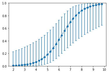
On our GitHub page, we provide a Jupyter notebook that contains some minimal code extending the SKLearn LogisticRegression class. This extension makes use of the results presented here and allows for class probability confidence intervals to be returned for individual test points. In the notebook, we apply the algorithm to the SKLearn Iris dataset. The figure at right illustrates the output of the algorithm along a particular cut through the Iris data set parameter space. The y-axis represents the probability of a given test point belong to Iris class $1$. The error bars in the plot provide insight that is completely missed when considering the point estimates only. For example, notice that the error bars are quite large for each of the far right points, despite the fact that the point estimates there are each near $1$. Without the error bars, the high probability of these point estimates might easily be misinterpreted as implying high model confidence.
Our derivations below rely on some prerequisites: Properties of covariance matrices, the multivariate Cramer-Rao theorem, and properties of maximum likelihood estimators. These concepts are covered in two of our prior posts [$1$, $2$].
Optimization by gradient descent
In this section, we derive expressions for the gradient of the negative-log likelihood loss function and also demonstrate that this loss is everywhere convex. The latter result is important because it implies that gradient descent can be used to find the maximum likelihood solution.
Again, to fit the logistic model to a training set, our aim is to find — and also to set the parameter vector to — the maximum likelihood value. Assuming the training set samples are independent, the likelihood of observing the training set labels is given by\begin{eqnarray}L &\equiv& \prod_i p(y_i \vert \vec{x}i) \&=& \prod{i: y_i = 1} \frac{1}{1 + e^{-\vec{\beta} \cdot \vec{x}i}} \prod{i: y_i = 0} \frac{1}{1 + e^{\vec{\beta} \cdot \vec{x}i}}.\tag{3} \label{likelihood}\end{eqnarray}Maximizing this is equivalent to minimizing its negative logarithm — a cost function that is somewhat easier to work with,\begin{eqnarray}J &\equiv & -\log L \&=& \sum{{i: y_i = 1 }} \log \left (1 + e^{- \vec{\beta} \cdot \vec{x}i } \right ) + \sum{{i: y_i = 0 }} \log \left (1 + e^{\vec{\beta} \cdot \vec{x}_i } \right ).\tag{4} \label{costfunction}\end{eqnarray}The maximum-likelihood solution, $\vec{\beta}^$, is that coefficient vector that minimizes the above. Note that $\vec{\beta}^$ will be a function of the random sample, and so will itself be a random variable — characterized by a distribution having some mean value, covariance, etc. Given enough samples, a theorem on maximum-likelihood asymptotics (Cramer-Rao) guarantees that this distribution will be unbiased — i.e., it will have mean value given by the correct parameter values — and will also be of minimal covariance [$1$]. This theorem is one of the main results motivating use of the maximum-likelihood solution.
Because $J$ is convex (demonstrated below), the logistic regression maximum-likelihood solution can always be found by gradient descent. That is, one need only iteratively update $\vec{\beta}$ in the direction of the negative $\vec{\beta}$-gradient of $J$, which is\begin{eqnarray}– \nabla_{\vec{\beta}} J &=& \sum_{{i: y_i = 1 }}\vec{x}i \frac{ e^{- \vec{\beta} \cdot \vec{x}_i } }{1 + e^{- \vec{\beta} \cdot \vec{x}_i }}– \sum{{i: y_i = 0 }} \vec{x}i \frac{ e^{\vec{\beta} \cdot \vec{x}_i }}{1 + e^{\vec{\beta} \cdot \vec{x}_i } } \&\equiv& \sum{{i: y_i = 1 }}\vec{x}i p(y=0 \vert \vec{x}_i)-\sum{{i: y_i = 0 }} \vec{x}_i p(y= 1 \vert \vec{x}_i). \tag{5} \label{gradient}\end{eqnarray}Notice that the terms that contribute the most here are those that are most strongly misclassified — i.e., those where the model’s predicted probability for the observed class is very low. For example, a point with true label $y=1$ but large model $p(y=0 \vert \vec{x})$ will contribute a significant push on $\vec{\beta}$ in the direction of $\vec{x}$ — so that the model will be more likely to predict $y=1$ at this point going forward. Notice that the contribution of a term above is also proportional to the length of its feature vector — training points further from the origin have a stronger impact on the optimization process than those near the origin (at fixed classification difficulty).
The Hessian (second partial derivative) matrix of the cost function follows from taking a second gradient of the above. With a little algebra, one can show that this has $i-j$ component given by,\begin{eqnarray}H(J){ij} &\equiv& -\partial{\beta_j} \partial_{\beta_i} \log L \&=& \sum_k x_{k; i} x_{k; j} p(y= 0 \vert \vec{x}k) p(y= 1 \vert \vec{x}_k). \tag{6} \label{Hessian}\end{eqnarray}We can prove that this is positive semi-definite using the fact that a matrix $M$ is necessarily positive semi-definite if $\vec{s}^T \cdot M \cdot \vec{s} \geq 0$ for all real $\vec{s}$ [$2$]. Dotting our Hessian above on both sides by an arbitrary vector $\vec{s}$, we obtain\begin{eqnarray}\vec{s}^T \cdot H \cdot \vec{s} &\equiv & \sum_k \sum{ij} s_i x_{k; i} x_{k; j} s_j p(y= 0 \vert \vec{x}_k) p(y= 1 \vert \vec{x}_k) \&=& \sum_k \vert \vec{s} \cdot \vec{x}_k \vert^2 p(y= 0 \vert \vec{x}_k) p(y= 1 \vert \vec{x}_k) \geq 0.\tag{7} \label{convex}\end{eqnarray}The last form follows from the fact that both $ p(y= 0 \vert \vec{x}_k) $ and $ p(y= 1 \vert \vec{x}_k) $ are non-negative. This holds for any $\vec{\beta}$ and any $\vec{s}$, which implies that our Hessian is everywhere positive semi-definite. Because of this, convex optimization strategies — e.g., gradient descent — can always be applied to find the global maximum-likelihood solution.
Coefficient uncertainty and significance tests
The solution $\vec{\beta}^$ that minimizes $J$ — which can be found by gradient descent — is a maximum likelihood estimate. In the asymptotic limit of a large number of samples, maximum-likelihood parameter estimates satisfy the Cramer-Rao lower bound [$2$]. That is, the parameter covariance matrix satisfies [$3$],\begin{eqnarray}\text{cov}(\vec{\beta}^, \vec{\beta}^*) &\sim& H(J)^{-1} \&\approx & \frac{1}{\sum_k \vec{x}{k} \vec{x}{k}^T p(y= 0 \vert \vec{x}_k) p(y= 1 \vert \vec{x}_k)}.\tag{8} \label{covariance}\end{eqnarray}Notice that the covariance matrix will be small if the denominator above is large. Along a given direction, this requires that the training set contains samples over a wide range of values in that direction (we discuss this at some length in the analogous section of our post on Linear Regression [$4$]). For a term to contribute in the denominator, the model must also have some confusion about its values: If there are no difficult-to-classify training examples, this means that there are no examples near the decision boundary. When this occurs, there will necessarily be a lot of flexibility in where the decision boundary is placed, resulting in large parameter variances.
Although the form above only holds in the asymptotic limit, we can always use it to approximate the true covariance matrix — keeping in mind that the accuracy of the approximation will degrade when working with small training sets. For example, using (\ref{covariance}), the asymptotic variance for a single parameter can be approximated by\begin{eqnarray}\tag{9} \label{single_cov}\sigma^2{\beta^*_i} = \text{cov}(\vec{\beta}^*, \vec{\beta}^*){ii}.\end{eqnarray}In the asymptotic limit, the maximum-likelihood parameters will be Normally-distributed [$1$], so we can provide confidence intervals for the parameters as\begin{eqnarray}\tag{10} \label{parameter_interval}\beta_i \in \left ( \beta^_i – z \sigma_{\beta^i}, \beta_i^* + z \sigma{\beta^*_i} \right),\end{eqnarray}where the value of $z$ sets the size of the interval. For example, choosing $z = 2$ gives an interval construction procedure that will cover the true value approximately $95\%$ of the time — a result of Normal statistics [$5$]. Checking which intervals do not cross zero provides a method for identifying which features contribute significantly to a given fit.
Prediction confidence intervals
The probability of class $1$ for a test point $\vec{x}$ is given by (\ref{model1}). Notice that this depends on $\vec{x}$ and $\vec{\beta}$ only through the dot product $\vec{x} \cdot \vec{\beta}$. At fixed $\vec{x}$, the variance (uncertainty) in this dot product follows from the coefficient covariance matrix above: We have [$2$],\begin{eqnarray}\tag{11} \label{logit_var}\sigma^2{\vec{x} \cdot \vec{\beta}} \equiv \vec{x}^T \cdot \text{cov}(\vec{\beta}^*, \vec{\beta}^*) \cdot \vec{x}.\end{eqnarray}With this result, we can obtain an expression for the confidence interval for the dot product, or equivalently a confidence interval for the class probability. For example, the asymptotic interval for class $1$ probability is given by\begin{eqnarray}\tag{12} \label{prob_interval}p(y=1 \vert \vec{x}) \in \left ( \frac{1}{1 + e^{- \vec{x} \cdot \vec{\beta}^* + z \sigma{\vec{x} \cdot \vec{\beta}^}}}, \frac{1}{1 + e^{- \vec{x} \cdot \vec{\beta}^ – z \sigma_{\vec{x} \cdot \vec{\beta}^}}} \right),\end{eqnarray}where $z$ again sets the size of the interval as above ($z=2$ gives a $95\%$ confidence interval, etc. [$5$]), and $\sigma_{\vec{x} \cdot \vec{\beta}^}$ is obtained from (\ref{covariance}) and (\ref{logit_var}).
The results (\ref{covariance}), (\ref{logit_var}), and (\ref{prob_interval}) are used in our Jupyter notebook. There we provide code for a minimal Logistic Regression class implementation that returns both point estimates and prediction confidence intervals for each test point. We used this code to generate the plot shown in the post introduction. Again, the code can be downloaded here if you are interested in trying it out.
Summary
In this note, we have 1) reviewed how to fit a logistic regression model to a binary data set for classification purposes, and 2) have derived the expressions needed to return class membership probability confidence intervals for test points.
Confidence intervals are typically not available for many out-of-the-box machine learning models, despite the fact that intervals can often provide significant utility. The fact that logistic regression allows for meaningful error bars to be returned with relative ease is therefore a notable, advantageous property.
Footnotes
[$1$] Our notes on the maximum-likelihood estimators can be found here.
[$2$] Our notes on covariance matrices and the multivariate Cramer-Rao theorem can be found here.
[$3$] The Cramer-Rao identity [$2$] states that covariance matrix of the maximum-likelihood estimators approaches the Hessian matrix of the log-likelihood, evaluated at their true values. Here, we approximate this by evaluating the Hessian at the maximum-likelihood point estimate.
[$4$] Our notes on linear regression can be found here.
[$5$] Our notes on Normal distributions can be found here.