Whenever you spot a trend plotted against time, you would be looking at a time series. The de facto choice for studying financial market performance and weather forecasts, time series are one of the most pervasive analysis techniques because of its inextricable relation to time—we are always interested to foretell the future.
Temporal Dependent Models
One intuitive way to make forecasts would be to refer to recent time points. Today’s stock prices would likely be more similar to yesterday’s prices than those from five years ago. Hence, we would give more weight to recent than to older prices in predicting today’s price. These correlations between past and present values demonstrate temporal dependence, which forms the basis of a popular time series analysis technique called ARIMA (Autoregressive Integrated Moving Average). ARIMA accounts for both seasonal variability and one-off ‘shocks’ in the past to make future predictions.
However, ARIMA makes rigid assumptions. To use ARIMA, trends should have regular periods, as well as constant mean and variance. If, for instance, we would like to analyze an increasing trend, we have to first apply a transformation to the trend so that it is no longer increasing but stationary. Moreover, ARIMA cannot work if we have missing data.
To avoid having to squeeze our data into a mould, we could consider an alternative such as neural networks. Long short-term memory (LSTM) networks are a type of neural networks that builds models based on temporal dependence. While highly accurate, neural networks suffer from a lack of interpretability—it is difficult to identify the model components that lead to specific predictions.
General Additive Models
Besides using correlations between values from similar time points, we could take a step back to model overall trends. A time series could be seen as a summation of individual trends. Take, for instance, google search trends for persimmons, a type of fruit.
From the Figure 1, we can infer that persimmons are probably seasonal. With its supply peaking in November, grocery shoppers might be prompted to google for nutrition facts or recipes for persimmons.
Moreover, google searches for persimmons are also growing more frequent over the years.
Therefore, google search trends for persimmons could well be modeled by adding a seasonal trend to an increasing growth trend, in what’s called a generalized additive model (GAM).
The principle behind GAMs is similar to that of regression, except that instead of summing effects of individual predictors, GAMs are a sum of smooth functions. Functions allow us to model more complex patterns, and they can be averaged to obtain smoothed curves that are more generalizable.
Because GAMs are based on functions rather than variables, they are not restricted by the linearity assumption in regression that requires predictor and outcome variables to move in a straight line. Furthermore, unlike in neural networks, we can isolate and study effects of individual functions in a GAM on resulting predictions.
In this tutorial, we will:
-
See an example of how GAM is used.
-
Learn how functions in a GAM are identified through backfitting.
-
Learn how to validate a time series model.
Example: Saving Daylight Time
People who have lived in regions with four seasons would know a fact: you get less sunshine during winter than in summer. To compensate for this, some countries move their clocks forward by an hour during summer months, scheduling more sunshine for evening outdoor activities and hopefully decreasing energy used for heating and lighting at home. This practice of advancing clocks during summer is called daylight saving time (DST), and was first implemented in the 1900s.
Actual benefits of DST are nonetheless controversial. Notably, DST has been shown to disrupt sleep patterns that affect work performance and even cause accidents. Hence, whenever it is time to adjust their clocks, people might be prompted to question the rationale for DST, and Wikipedia is one source for answers.
To study trends for DST page views, we first used a Python script to extract the data from a Wikipedia database. Page view counts from 2008 to 2015 were used. Next, we used a GAM package called Prophet published by Facebook researchers to conduct our time series analysis in Python. The package is also available in R.
The Prophet package is user-friendly, allowing us to specify different types of functions comprising the resulting GAM trend. There are three main types of functions:
Overall Growth. This can be modeled either as a straight (linear) or slightly curved (logistic) trend. In this analysis, we use the default linear growth model.
Seasonal Variations. This is modeled using Fourier series, which is simply a way to approximate periodic functions. The exact functions are derived using a process known as backfitting, to be explained in the next section. We can specify if we anticipate weekly or/and annual trends to be present. In this analysis, we include both—a weekly trend is plausible based on past studies that show less internet activity on weekends when people are likely to be outdoors, while a yearly trend might coincide with the biannual clock-turning exercise.
Special Events. Besides modeling regular trends, we should also account for one-off events. This includes any phenomenon, be it policy announcements or natural disasters, that would add ripples to an otherwise smooth trend. If we do not account for irregular events, the GAM might mistake them to be persistent occurrences and their effects would be erroneously propagated.
In our analysis, special events included exact dates when US clocks are turned back and forth. We can also specify windows before and after each event where we expect significant effects. Before each time switch, for instance, online searches on DST might start increasing. But search behavior after the time switch might differ, depending on whether the clock is winded forward or backward: people might be more likely to search online for why their sleep is shortchanged, but not when they get extra snooze. Besides clock-turning dates, we also included major DST-related events. In 2010, for example, protests erupted in Israel over an unusually early switch back to winter time due to differences between the Hebrew and solar calendar. Events included in our analysis can be found in the code.
In addition to the above, the Prophet package also requires us to specify prior values, which determine how sensitive our trend line should be to changes in data values. Higher sensitivity results in more jagged trends, which could affect generalizability to future values. Priors can be tuned when we validate our model, which we will see later in this tutorial.
For now, we can proceed to fit a GAM. Figure 3 shows the resulting functions for overall growth, special events, and seasonal variations:

Figure 3. Functions comprising the GAM predicting page views of DST Wikipedia article. In the first two graphs for overall trend and special events (i.e. ‘holidays’), the x-axis is labeled ‘ds’, which stands for ‘date stamp’. Duplicate year labels appear because the grid lines do not coincide uniformly with the same date in each year.
We can see that overall page views of the DST Wikipedia article is generally decreasing across the years, possibly due to competing online sources explaining DST. We can also observe how spikes in page views that coincide with special events have been accounted for. Weekly trends reveal that people are most likely to read about DST on Mondays, and least likely on weekends. And finally, annual trends show that page views peak in end-March and end-October, periods when time switches occur.
It is convenient how we don’t need to know the exact predictor functions to include in a GAM. Instead, we only have to specify a few constraints and the best functions would be derived automatically for us. How does GAM do this?
Backfitting Algorithm
To find the best trend line that fits the data, GAM uses a procedure known as backfitting. Backfitting is a process that tweaks the functions in a GAM iteratively so that they produce a trend line that minimizes prediction errors. A simple example can be used to illustrate this process.
Suppose we have the following data:
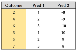
Figure 4. Example dataset, consisting of two predictors and an outcome variable.
Our aim is to find suitable functions to apply to the predictors, so that we can predict the outcome accurately.
First, we work on finding a function for Predictor 1. A good initial guess might be to multiply it by 2:
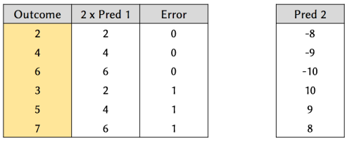
Figure 5. Results of a model that applies a ‘multiply by 2’ function to Predictor 1.
From Figure 5, we can see that by applying a ‘multiply by 2’ function to Predictor 1, we can predict 50% of the outcome perfectly. However, there is still room for improvement.
Next, we work on finding a function for Predictor 2. By analyzing the prediction errors from fitting Predictor 1’s function, we can see that it is possible to achieve 100% accuracy by simply adding 1 to the outcome whenever Predictor 2 has a positive value, and doing nothing otherwise (i.e. signmoid function).
This is the gist of a backfitting process, which is summed up by the following steps:
Step 0: Define a function for one predictor and calculate the resulting error.
Step 1: Derive a function for the next predictor that best reduces the error.
Step 2: Repeat Step 1 for all predictors, and further repeating the cycle to re-assess their functions if necessary, until prediction error cannot be further minimized.
Now that we’ve fitted our model, we need to put it to the test: is it able to forecast future values accurately?
Validating a Time Series Model
Cross-validation is the go-to technique for assessing a model’s effectiveness in predicting future values. However, time series models are one exception where cross-validation would not work.
Recall that cross-validation involves dividing the dataset into random subsamples that are used to train and test the model repeatedly. Crucially, data points used in training samples must be independent of those in the test sample. But this is impossible in time series, because data points are time-dependent, so data in the training set would still carry time-based associations with the test set data. This calls for different techniques to validate time series models.
Instead of sampling our data points across time, we can slice them based on time segments. If we want to test our model’s forecast accuracy one year into the future (i.e. forecast horizon), we can divide our dataset into training segments of one year (or longer), and use each segment to predict values in its subsequent year. This technique is called simulated historical forecasts. As a guide, if our forecast horizon is one year, then we should make simulated forecasts every half a year. Results of 11 simulated forecasts for DST’s Wikipedia page views are shown in Figure 6.
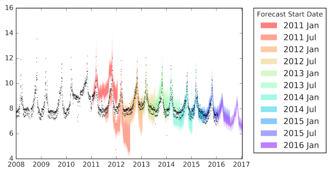
Figure 6. Simulated historical forecasts of DST’s Wikipedia page views.
In Figure 6, the forecast horizon was one year, and each training segment comprised three years worth of data. For example, the first forecast band (in red) uses data from January 2008 to December 2010 to predict views for January 2011 – December 2011. We can see that apart from the first two simulated forecasts, which were misled by the unusually high page activity in 2010, predictions generally overlapped well with actual values.
To better assess the model’s accuracy, we can take the mean prediction error from all 11 simulated forecasts and plot that against the forecast horizon, as shown in Figure 7. Notice how error increases as we try to forecast further into the future.
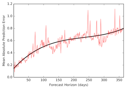
Figure 7. Prediction errors across the forecast horizon. The red line represents the mean absolute error across the 11 simulated forecasts, while the black line is a smoothed trend of that error.
Recall that one of the parameters we need to tune is the values of priors, which determine how sensitive our trend should be to changes in data values. One way to do this is to try different parameter values and compare the resulting errors via plots such as Figure 8. As we can see, an overly-large prior leads to a less generalizable trend, and thus larger errors.

Figure 8. Comparison of prediction errors resulting from different prior values.
Besides tuning priors, we can also tweak settings for the base growth model, seasonality trends, and special events. Visualizing our data also helps us to identify and remove outliers. For instance, we can improve predictions by excluding data from 2010, during which page view counts were unusually high.
Limitations
As you might have surmised, having more training data in a time series need not necessarily lead to more accurate models. Anomalous values or rapidly changing trends could upend any prediction efforts. Worse still, sudden shocks that permanently affect a time series could also render all past data as irrelevant.
Therefore, time series analysis works best for trends that are steady and systematic, for which we can assess with visualizations.
Summary
-
Time series analysis is a technique to derive a trend across time, which might be used to predict future values. A Generalized Additive Model (GAM) does this by identifying and summing multiple functions that results in a trend line that best fits the data.
-
Functions in a GAM can be identified using the backfitting algorithm, which fits and tweaks functions iteratively in order to reduce prediction error.
-
Time series analysis works best for trends that are steady and systematic.
Did you learn something useful today? We would be glad to inform you when we have new tutorials, so that your learning continues!
Sign up below to get bite-sized tutorials delivered to your inbox:
![]()
Copyright © 2015-Present Algobeans.com. All rights reserved. Be a cool bean.
References
Like this:
Like Loading…
Related