Sometimes in statistics, one knows certain facts with absolute certainty about a distribution. For example, let $@ t $@ represent the time delay between an event occurring and the same event being detected. I don’t know very much about the distribution of times, but one thing I can say with certainty is that $@ t > 0 $@; an event can only be detected after it occurs.
In general, when we don’t know the distribution of a variable at all, it’s a problem for nonparametric statistics. One popular technique is Kernel Density Estimation. Gaussian KDE builds a smooth density function from a discrete set of points by dropping a Gaussian kernel at the location of each point; provided the width of the Gaussians shrinks appropriately as the data size increases, and the true PDF is appropriately smooth, this can be proven to approximate the true PDF.
However, the problem with Gaussian KDE is that it doesn’t respect boundaries.
Although we know apriori that every data point in this data set is contained in [0,1] (because I generated the data that way), unfortunately the Gaussian KDE approximation does not respect this. By graphing the data together with the estimate PDF, we discover a non-zero probability of finding data points below zero or above one:
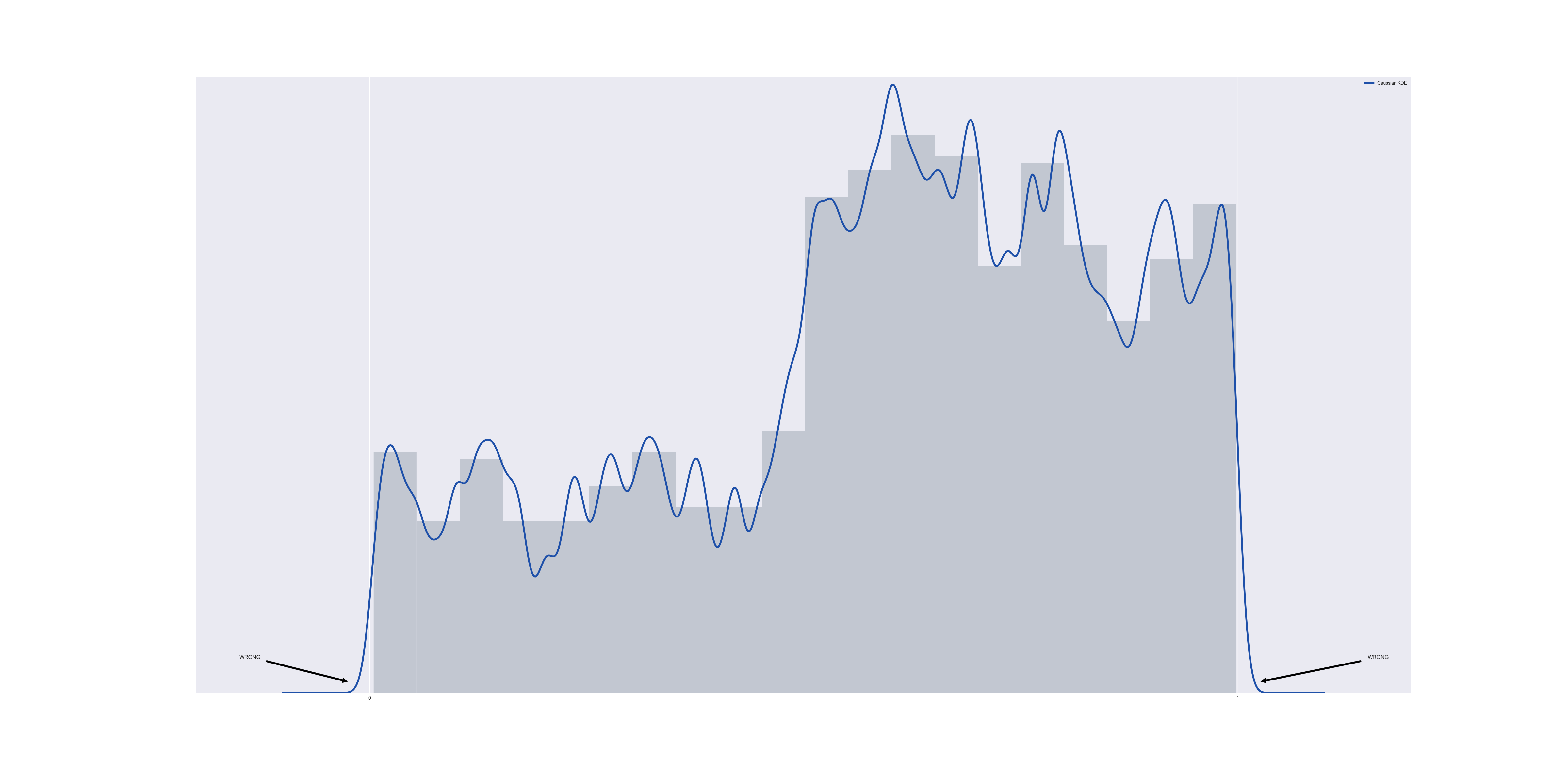
The problem is that although we know the data set is bounded below by $@ t = 0 $@, we are unable to communicate this information to the gaussian KDE.
Lets consider a very simple data set, one with two data points at $@ t = 0.1 $@ and $@ t = 0.3 $@ respectively. If we run a gaussian KDE on this, we obtain:
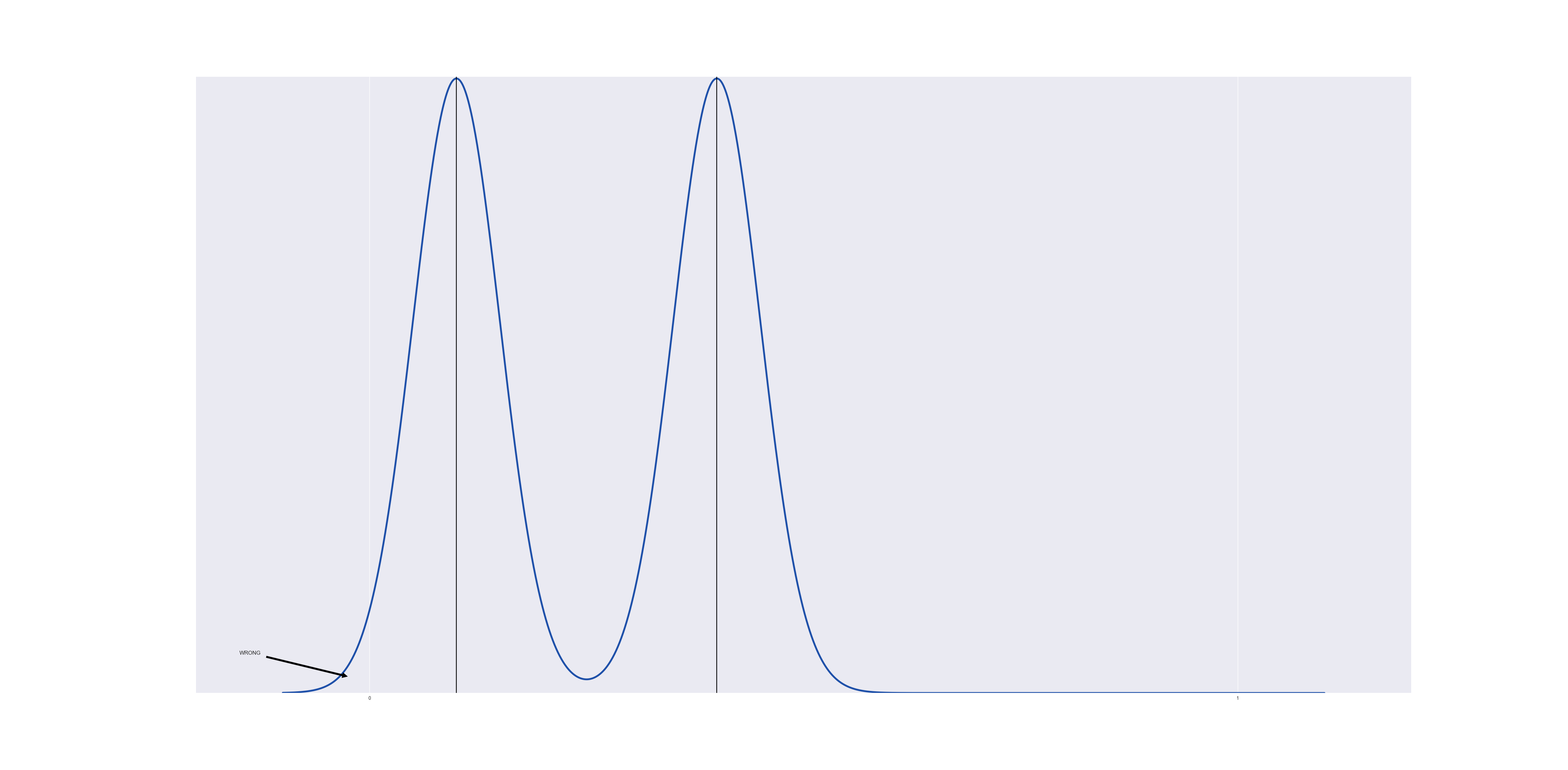
The gaussian near $@ t=0 $@ overspills into the region below $@ t < 0 $@.
Kernel Density Estimation that Respects Boundaries
The way to resolve this issue is to replace the Gaussian kernel with a kernel that does respect boundaries. For example, if we wish to respect boundaries of [0,1], we can use a beta distribution. Because the variance of a beta distribution is an important parameter, we’ll try and choose a beta distribution with the same variance as a comparable gaussian kernel.
The beta distribution takes two parameters, $@ \alpha $@ and $@ \beta$@, has mean $@ \alpha/(\alpha+\beta) $@ and variance $@ \alpha\beta/((\alpha+\beta)^2(\alpha+\beta+1)) $@.
So what we’ll do is choose a bandwidth parameter $@ K $@, set $@ \alpha = dK $@ and $@ \beta = (1-d)K $@ for a data point $@ d $@. Then the mean will be $@ \alpha/(\alpha+\beta) = dK/(dK+(1-d)K) = d $@. The value $@ K $@ can then be chosen so as to make the variance equal to a gaussian, i.e.:
K = \frac{d(1-d)}{V} - 1 $@
(This calculation is done in the appendix.)
If we remain away from the boundary, a beta distribution approximates a gaussian very closely:
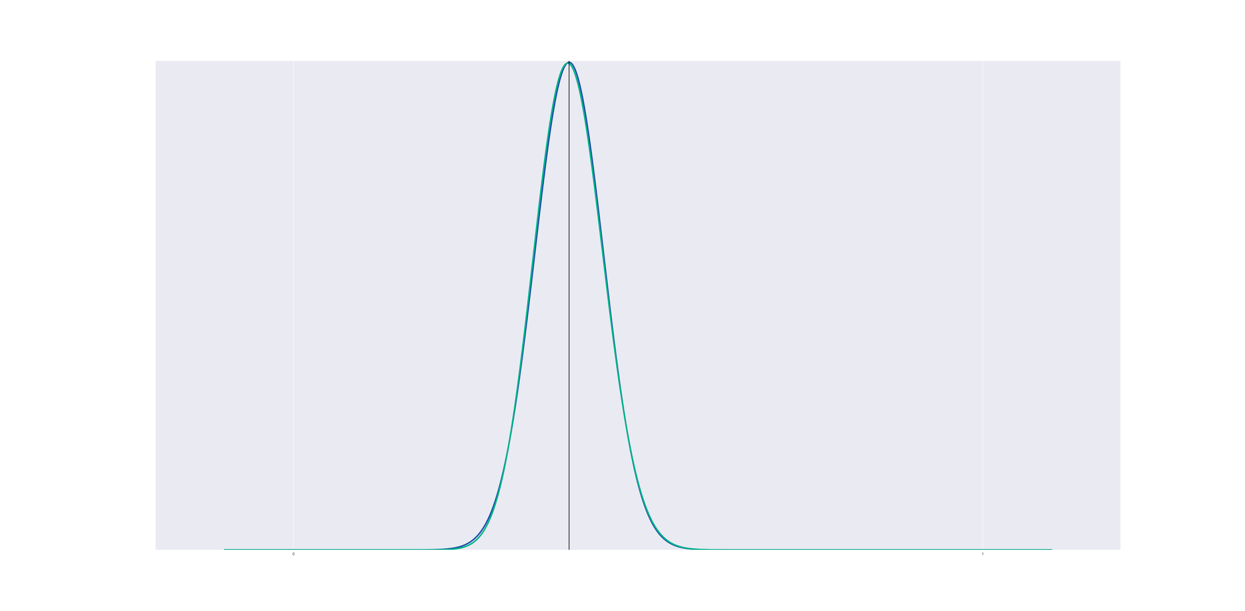
In this graph (and all the graphs to follow), the blue line represents a Gaussian KDE while the green line represents the Beta KDE.
But if we center a gaussian and a beta distribution at a point near the boundary, the beta distribution changes shape to avoid crossing the line $@ x=0 $@:
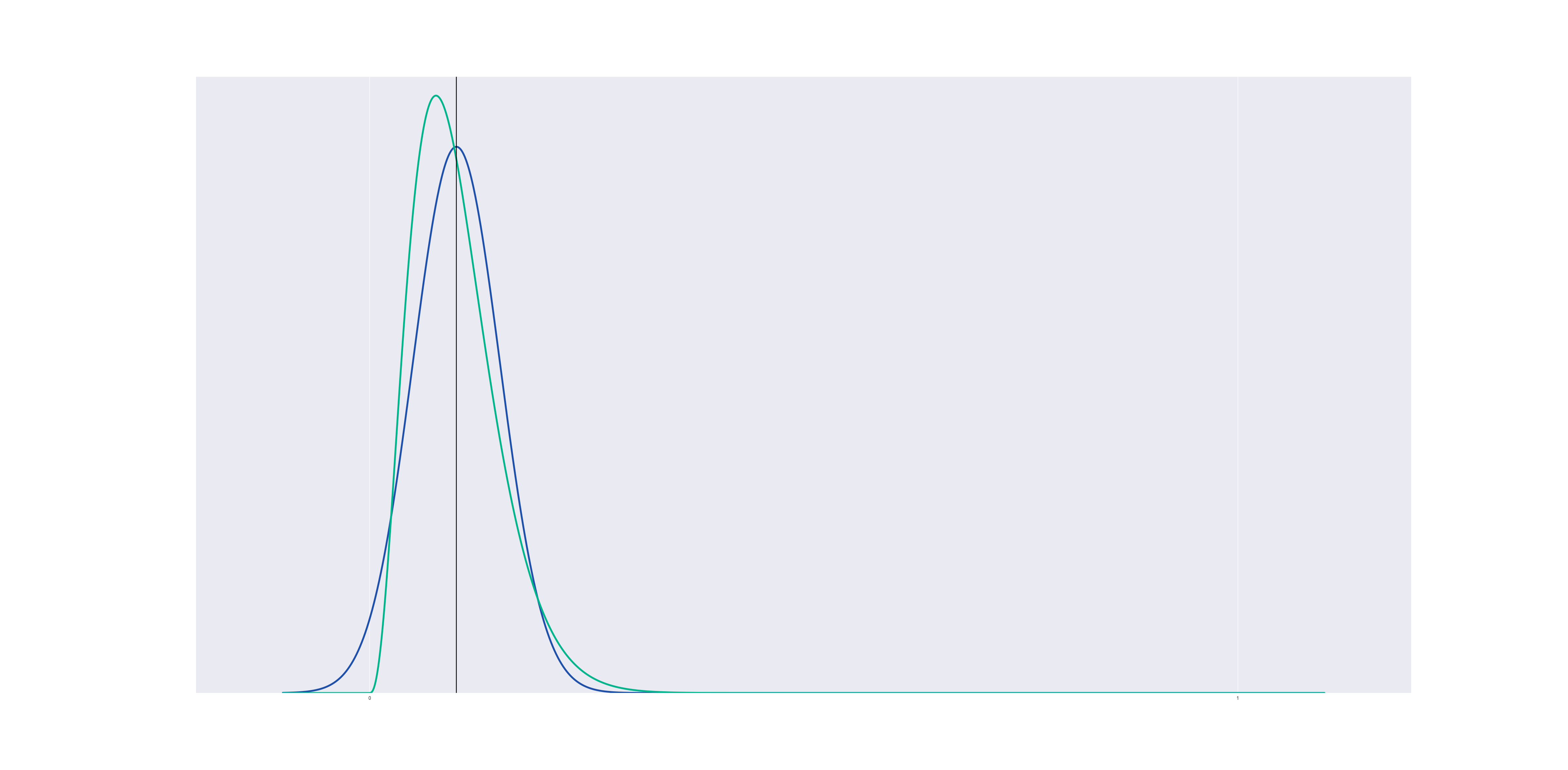
Now suppose we run a kernel density estimation using beta distributions, centered at the data points. The result is a lot like gaussian KDE, but it respects the boundary:
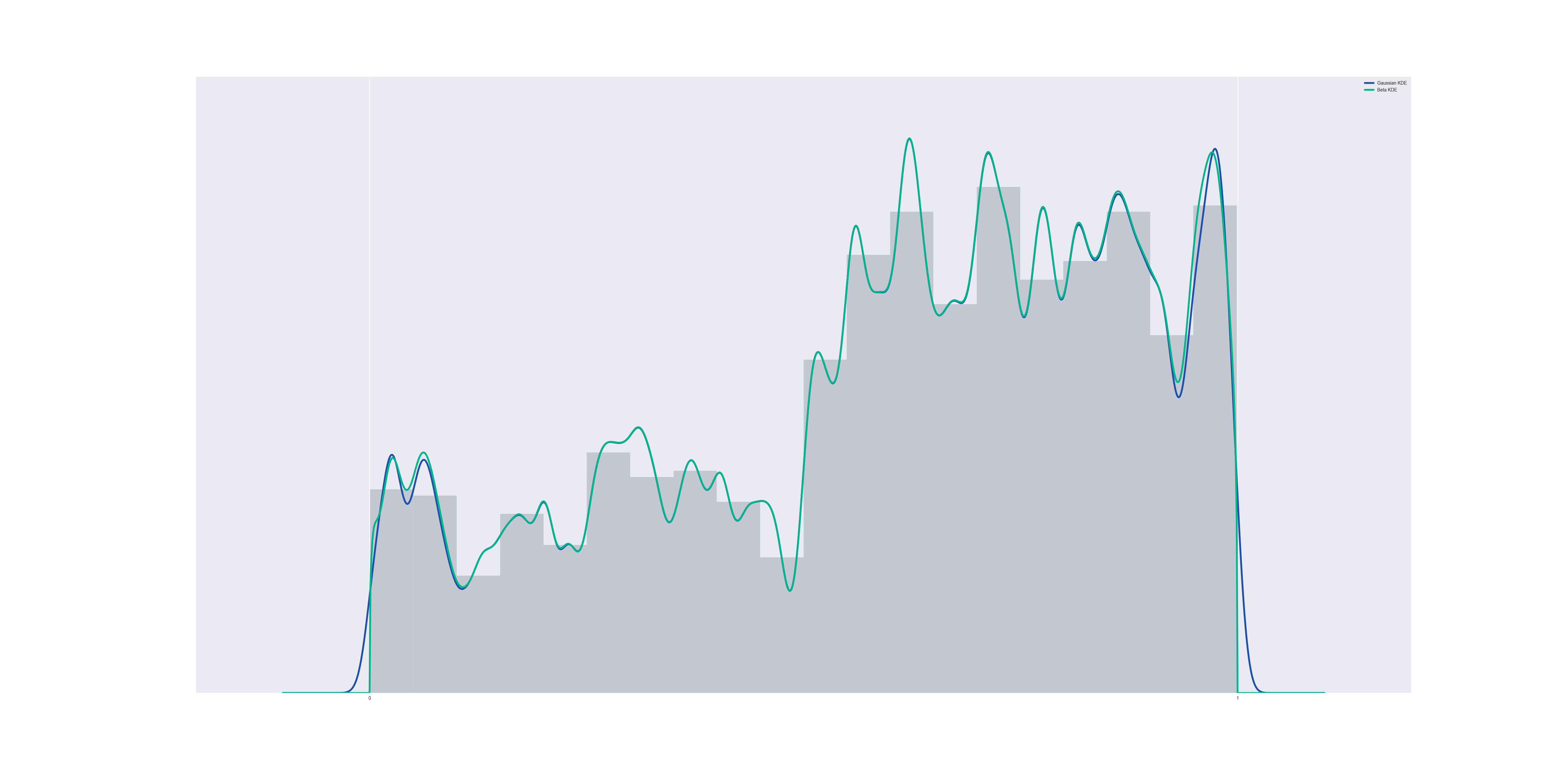
The code to generate this is the following (for a 1000-element data set, and a kernel bandwidth of 0.01):
Generalizations
A generalization of this idea can be used on the unit simplex, i.e. the set of vectors with $@ \vec{d}_i \geq 0 $@ and $@ \sum_i \vec{d}_i = 1 $@.
| Consider a data point $@ \vec{d} $@ on the unit simplex. Given a large parameter $@ K $@, one can define $@ \vec{\alpha} = K\vec{d} $@ and use a $@ \textrm{Dirichlet}( K\vec{d}) $@ distribution in the exact same way we used a beta distribution above. Recall that a Dirichlet distribution has mean $@ \vec{\alpha} / | \vec{\alpha} | _{l^1} = \vec{d} $@ if $@ \alpha = K\vec{d} $@. By making $@ K $@ sufficiently large, the variance (which is $@O(K^{-1})$@) will be small, so this Dirichlet distribution behaves the same way as the beta distribution above. |
This would allow us to run a KDE-like process on the unit simplex.
MCMC
Another situation which can arise is in MCMC. In a Bayesian nonparametric regression situation that I ran into recently, I needed a proposal distribution for vectors which I knew lived on the unit simplex. Given the old value $@ \vec{d} $@, I drew a proposed value given the exact distribution described above.
Conclusion
When using kernel approximations, don’t treat the process as a black box. One can often preserve valuable properties and get more accurate results simply by making model-based tweaks to the kernel. This is a very important fact I learned in my academic career as a (computational) harmonic analyst, but which I don’t see the data science community adopting.
Special thanks to Lisa Mahapatra for massively improving my data visualizations.
Appendix: Where does the formula for K come from?
Consider a gaussian with variance $@ V $@. We want to construct a beta distribution with the same variance, centered at the point $@ d $@. Note that for a beta distribution with parameters $@ \alpha, \beta $@, the variance is:
\textrm{Var} = \frac{ \alpha \beta } { (\alpha + \beta)^2(\alpha + \beta + 1) } $@
(I’m taking these identities from le wik.)
Now let $@ \alpha = K d $@ and $@ \beta = K(1-d) $@. Then we obtain the variance:
\textrm{Var} = \frac{ K^2 d (1-d) } { (K d + K(1-d))^2(Kd + K(1-d) + 1) } = \frac{ K^2 d (1-d) } { K^2(K + 1) } = \frac{ d(1-d) }{K+1} $@
Now suppose we wanted the variance of a beta distribution to be $@ V $@, then we would set this equal to $@ V $@ and solve for $@ K $@. The result is:
K = \frac{d(1-d)}{V} - 1 $@
There is one important fact to note. For $@ d < V $@, the resulting $@ K $@ will actually become negative. This will result in a singular beta distribution. So to get a non-singular PDF, we need to bound $@ K $@ below by zero; in practice I’ve found choosing $@ K = \max(\frac{d(1-d)}{V} - 1, 100) $@ works reasonably well.
Unregularized vs regularized
If we do not impose regularization conditions, then if any data points exist which make $@ K $@ negative, the pdf becomes singular at $@ x=0 $@ and/or $@ x=1 $@.
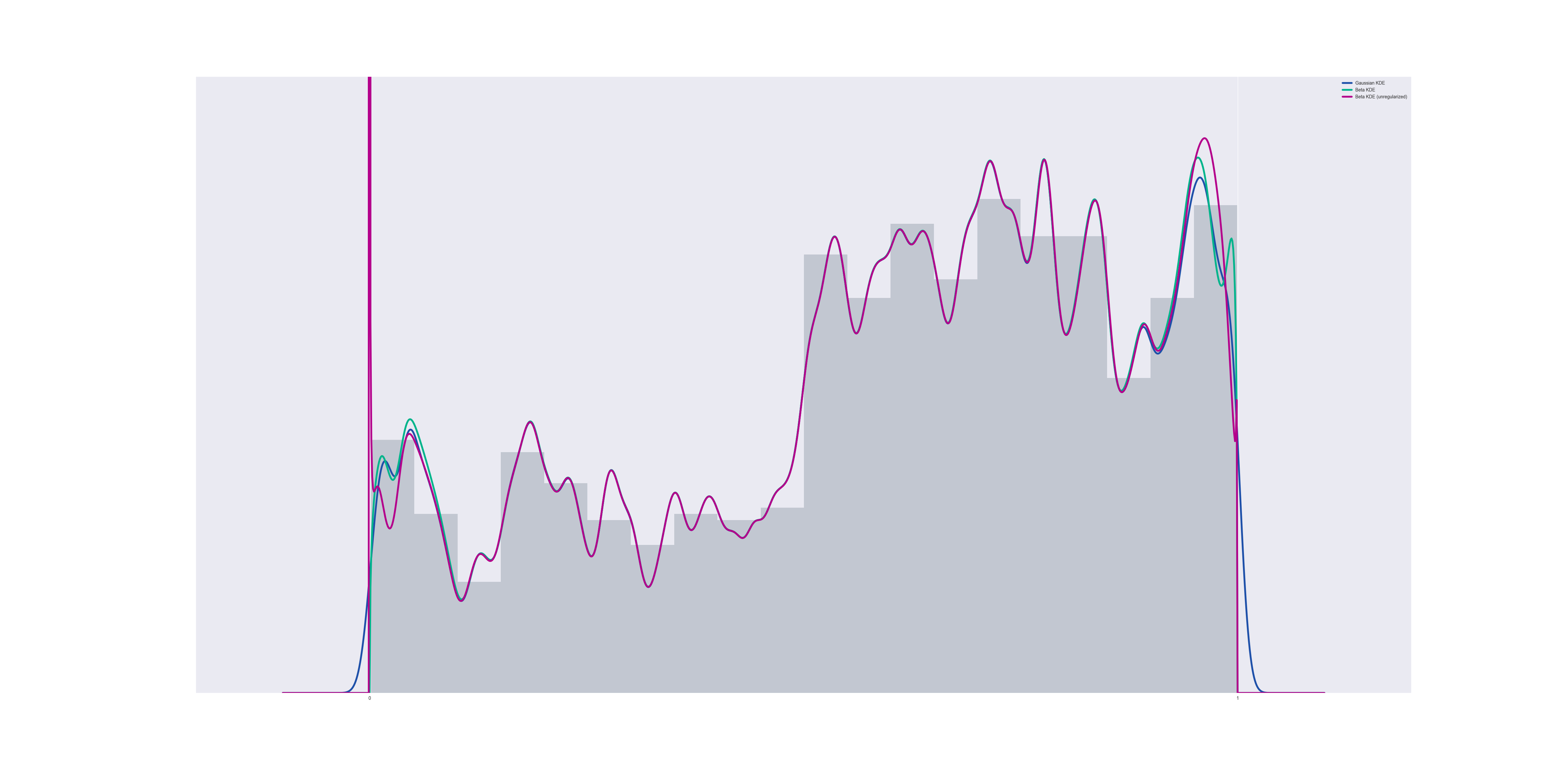
However, the CDF of the distribution does NOT become singular, merely non-differentiable. The nature of the problem is that the PDF behaves like $@ x^K $@ for some $@ -1 < K < 0 $@ near $@ x=0 $@. This is an integrable singularity, and the CDF then behaves like $@ x^{K+1} $@ which is a continuous function.